As of January 2004 au.riversinfo.org is archived under Precision Info
RIVERSINFO AUSTRALIA ARCHIVE
This archive provides non stylised versions of selected reference documents (formerly) resident on au.riversinfo.org.
National River Health Program: Project S3/UCU
Jacob John. School of Environmental Biology, Curtin University of Technology
LWRRDC Occasional Paper 13/99. (Urban Subprogram, Report No. 6)
Foreword, Publication Information & Acknowledgements
Chapter 3: Materials and Methods
Appendix 1 Assortment of Sampling Sites
Appendix 2 Physico-Chemical Data Sheet spring/summer 1997
Appendix 3 Diatom Index Spread Sheet & Worked Out Examples
Appendix 4 Autumn/winter 1997 Dendrogram Based Upon Diatoms
Appendix 5 Correlation Coefficients of Diatom Species
Appendix 6 Two-Way Tables of Diatom Distribution and Sites
The metropolitan city of Perth has its beginning with the establishment of the Swan River Colony in 1829, around the Swan-Canning River estuary. Within the last 170 years the city has expanded with almost 1.4 million people inhabiting the metropolitan city impacting heavily on the ecology of the River system. Several natural streams discharging into the system have been drastically modified by intense urbanisation. The River system and its tributaries, streams and drains have been the recipients of nutrients, effluents, and waste water from the urban and rural catchments resulting in severe symptoms of eutrophication over the past several decades. While the rural catchments have been implicated in the eutrophication and pollution of the estuary, the contribution of urban catchments to the degradation of the system is relatively less known. Through urban catchment groups, and the Integrated Catchment Management Policy, the importance of urban streams and drains is just beginning to be recognised. The current project was aimed at developing a predictive model for biomonitoring the urban streams using diatoms as tools. The investigation lasting from 1996 to 1999 focussed on classification of the urban streams using water quality parameters and 'stream conditions' and subsequent development of a predictive model using diatoms as biomonitors.
Close to 180 sites were sampled in summer 1996, spring-summer 1997 and autumn-winter 1997 recording as many as 30 environmental variables. These sites represented most of the streams and drains (including 'concrete') in the urban and semi-rural areas of Perth. The sampling sites were established after analysing the historical data on water quality and catchment conditions, as well as from preliminary observations. A large number of 'reference sites' or 'relatively pristine sites' were required for the model. The semi-rural sites provided the best examples of reference sites, as they were least impacted by urbanisation. Diatom samples from both reference and impacted sites were collected using an artificial sampling device – the JJ Periphytometer.
All the sites were classified on the basis of seven environmental variables with the highest correlation coefficient with the sites, using the agglomerative hierarchical fusion method with flexible unweighted pair group mean averages (UPGMA) within the multivariate pattern analysis program PATN. The dendrogram with the sites clustered according to their similarity, was further analysed and the status of some of the sites revised, recognising a third group 'the Intermediates'.
Out of more than 200 species of diatoms recorded from the sampling sites, 57 species selected on the basis of their relative frequencies, were used for the classification of the sites to show the similarity in the distribution pattern of diatoms. Diatom assemblages with similar ecological preferences were clustered together. Discriminant function analysis showed that there was a high degree of concordance between the two classifications. Multi-dimensional Scaling (MDS) was employed for ordination of sites based on diatom assemblages. Environmental variables were related to the ordination with principal axis correlation. Stream conditions such as water table depth and percentage of native vegetation had significant correlation with pristine sites, where as, alkalinity, electrical conductivity, ground water salinity, catchment land use, riparian damage and colour had significant correlation coefficients with the impacted sites. The distribution pattern of diatoms were separated into three distinct groups: Reference, Monitoring and Intermediate – within the intermediate group, the brackish sites were further separated. Several indicator species were recognised on the basis of the correlation of the species to the sites.
A two-way table with the distribution pattern of diatoms constrained on the site groups was generated. This table can be used to assess the health of any site chosen. The diatom assemblages of the test site can be added to the horizontal rows with their relative frequency. The test site then may be clustered with Impacted or Reference or Intermediate groups. In this way an assessment of its health may be made.
Based upon the indicator species for Reference and Impacted sites, a diatom index with predictive power has been designed. The health of any site can be assessed by providing the information on the relative frequency of diatom species present in the site. The predictive model was derived from the data collected from spring-summer 1997 but was successfully tested on winter samples 1997. The relatively high universality of diatom species distribution, makes them ideal biomonitors at the regional and national level.
The distribution pattern of diatoms in the urban streams and drains in the metropolitan city of Perth was highly correlated with the environmental factors associated with the ecological integrity and stream conditions. The predictive model developed in this project has the potential to be adapted for use in other urban areas of Australia.
This report describes the outcomes of a research project conducted under the Urban Research and Development sub-program of the National River Health Program (NRHP).
The NRHP is an on-going national program established in 1993, managed by the Land and Water Resources Research and Development Corporation (LWRRDC) and Environment Australia. Its mission is to improve the management of Australia's rivers and floodplains for their long-term health and ecological sustainability, through the following goals:
Urban streams and estuaries (i.e. those affected by runoff and discharges from urban areas) are an important subset of Australia's waterways. Most are degraded biologically, physically and chemically and therefore require appropriate methods to be developed for health assessment and management. The Urban R&D Sub-program, managed by the Water Services Association of Australia, comprises 8 research projects which were developed to meet research priorities for urban streams and estuaries within the goals of the NRHP and to complement existing NRHP projects on non-urban rivers. Thus, research focuses on development of standardised methods for assessing the ecological health of urban streams and estuaries which can be linked with data on water and sediment quality. The urban R&D projects commenced in 1996.
The definition of health in urban waterways used is "the ability to support and maintain a balanced, integrative, adaptive community of organisms having a species composition, diversity and functional organisation as comparable as practicable to that of natural habitats of the region".
The eight projects of the Urban Sub-Program are:
| Decision support system for management of urban streams | Dr John Anderson Southern Cross University, Lismore |
| RIVPACS (River InVertebrate Prediction and Classification System) for urban streams | Dr Peter Breen CRC for Freshwater Ecology, Monash University, Melbourne |
| DIPACS (Diatom Prediction and Classification System) for urban streams | Dr Jacob John
Curtin University, Perth |
| Sediment chemistry- macroinvertebrate fauna relationships in urban streams | Dr Nick O'Connor Water EcoScience, Melbourne |
| Classification of estuaries | Dr Peter Saenger Southern Cross University,Lismore |
| Literature review of ecological health assessment in estuaries | Mr David Deeley
Murdoch University, Perth |
| Estuarine health assessment using benthic macrofauna | Dr Gary Poore
Museum of Victoria, Melbourne |
| Estuarine eutrophication models | Dr John Parslow CSIRO Marine Laboratories, Hobart |
Diatom Prediction & Classification System for Urban Streams. A Model from Perth, Western Australia
National River Health Program: Project S3/UCU
Jacob John. School of Environmental Biology, Curtin University of Technology
LWRRDC Occasional Paper 13/99. (Urban Subprogram, Report No. 6)
May 2000
ISSN: 1320-0992
ISBN: 0-642-26763-4
Published by:
Land and Water Resources Research and Development Corporation
GPO Box 2182 Canberra ACT 2601
Telephone: (02) 6257 3379
Facsimile: (02) 6257 3420
Email: public@Iwwrrdc.gov.au
WebSite: www.lwrrdc.gov.au
© LWRRDC
Published Electronically on au.riversinfo.org by the Environmental Information Association (Incorporated) with the permission of LWRRDC and Environment Australia. Environment Australia assisted by providing copies of the manuscript for electronic publication. The Natural Heritage Trust provided project funds which were used to assist in publishing this material. In the case of variation between this document and the hard copy original the original takes precedence. (Bryan Hall).
The information contained in this publication has been published by LWRRDC to assist public knowledge and discussion and to help improve the sustainable management of land, water and vegetation. Where technical information has been prepared by or contributed by authors external to the Corporation, readers should contact the author(s), and conduct their own enquiries, before making use of that information.
I wish to express my gratitude to Dr John Langford (Executive Director, Water Services Association of Australia) for his constant encouragement in completing the project.
My thanks are extended to Water and Rivers Commission, WA for financial support for the water chemistry and Mr Jeff Kite (Water Resource section), Mr Malcolm Robb and Ms Mischa Cousins, from the Water and Rivers Commission.
I gratefully acknowledge the assistance of Mr Augustine Doronila with statistics and research assistants Ms Melanie Ward and Mr Chris John Siva for their field and lab work and general assistance in the project.
Finally, I wish to thank the School of Environmental Biology, Curtin University for providing facilities for the research project. Miss Erin Lowe, Miss Fiona Butson, my PhD students and Ms Jean Burgess of the School of Environmental Biology for their assistance in preparing this report.
Jacob John
School of Environmental Biology
Curtin University of Technology
GPO Box U 1987
Perth, WA
Email: RJACOBJO@cc.REMOVEcurtin.edu.au
Telephone: (08) 9266 7327
Facsimile: (08) 9266 2495
In February 2000, the Swan River Estuary, Western Australia was sieged by an outbreak of a fresh water toxic cyanobacterial bloom caused by a form of Microcystis aeruginosa. The river was closed to the public for two weeks. Although the Swan River had experienced algal blooms before, this was the first time the river was closed to the public. High concentrations of hepatotoxin in the bloom forced the closure. In previous years, there have been toxic cyanobacterial blooms in the fresh water section of the Canning River, the major tributary of the Swan River. Unusual heavy rains followed by large volumes of freshwater and nutrients washed into the estuary obviously altered the hydrology of the river. Most parts of the estuary which should have been saline had become fresh. Microcystis aeruginosa form flos-aquae which blooms in most of the urban and riverine wetlands including ditches and drains feeding into the Swan River, found a congenial haven in the Swan River. The unexpected fresh water blue green algal bloom provided a prime example of the influence of urban streams and drains on the water quality of the estuary – the pivotal centre of recreational life of the city of Perth – the home of almost 1.4 million people. Urban drains and streams, not only provide the conduit of transport of surface water and nutrients from the catchments, but also a few harmful algal blooms. Monitoring not only mere water quality, but assessment of the health of the drain and streams by suitable biota should be part of the management strategy of the estuarine systems.
This project was an attempt to investigate the relationship between stream conditions and the most diverse and numerous algae present in the urban drains and streams in the Perth metropolitan area – the diatoms. As all major cities of Australia are built around estuaries and rivers, this project may have wide application in other parts of Australia.
Freshwater rivers and streams have always been a convenient outlet for the removal of waste effluent. This is due to the fact that rivers flow downstream, effectively removing waste all the way. In the early stages of history, human settlements were made up of relatively small communities, and the human impact on rivers was minimal. The recent population explosion and increased utilisation of resources have resulted in the need for effluent control and treatment prior to discharge into waterways. Common river and stream uses include; fishing, drinking water, agriculture, irrigation, industrial abstraction, protection of flora and fauna, and water sports. These activities, all of which influence water quality to some degree, may only be perpetuated, if the water used is maintained sustainably (Sweeting 1994). The maintenance of sediment quality and stable riparian habitat are also required for full protection of freshwater ecosystems (Dobbs and Zabel 1994). An increase in public demands for environmental protection requires improved impact assessment of water resource schemes, especially for allocation of water to in-river needs (Petts et al.1995).
Modification of waterways such as damming or course redirection for irrigation purposes commonly occurs throughout the world. The specific impact of such manipulation on waterways is difficult to clarify (Allan 1995). In the last century, an increasing number of rivers have been significantly polluted due to human impact (Haslam 1994). The Rhone River in Switzerland was used mostly for rafting logs or stones in the early 19th century, and dykes and spurs were used to harness the flow. As a result, side arms were silted up, and lateral channels disappeared. This river has received increasing pollution loads over time, with industrialization and increased human settlement (Bravard et al.1992). Pollution is defined as any environmental state that is harmful to life, resulting from failure to maintain control of chemical, physical or biological consequences of human scientific, industrial or social habits (Sweeting 1994). The increased awareness of the effects of pollution on rivers, streams and seas may lead to an abatement of this problem by adoption of appropriate management strategies.
In natural streams, some areas may be polluted by natural causes e.g. in forested areas, high amounts of organic matter such as leaf litter may cause a large increase in organic matter, which effectively decreases dissolved oxygen. In New Zealand, high levels of arsenic released from sedimentary rocks of a particular area caused the death of large numbers of cattle in the 1960s (Lazaro 1979). Radon gas, emitted when uranium is broken down, may seep through the ground to springs, causing high levels of radioactivity (Haslam 1994).
The progressive eutrophication of a river system as it passes through cultivated and inhabited human settlements is inevitable. In densely populated (urban) areas, drainage and runoff may contribute excessive amounts of organic matter, causing pollution (Butcher 1947). Lenat and Crawford (1994) found that land use (forestry, agriculture or urbanisation) had a noticeable effect on the water quality and aquatic biota of three streams in North Carolina. Nutrient concentrations were found to be highest at the agricultural site, and available dissolved nitrogen was elevated in both the agricultural and urban sites. Maximum levels of metals (above the range considered safe) in the water column were recorded at the urban site, in particular, chromium, copper and lead. Ellis et al.(1986) also found that urban storm water carries heavy metals washed from roadsides, particularly cadmium and lead. Maximum concentrations of sediment metals were detected in the forested site. At the urban site, fish populations were characterised by low species richness, low biomass, and an absence of intolerant species.
Most of the pollution in our waterways may be attributed to human activity, in particular, urbanisation. Cultural eutrophication of water bodies is a world wide problem, which may be reversible. Urbanisation may be divided into four discrete stages; rural, early urban, middle urban and late urban. Rural areas are in a near-virgin state, under cultivation or in pasture. Early urban areas contain houses on large blocks, with most of the native vegetation remaining untouched, as in small suburbs and rural communities. Middle urban areas are identified by the presence of large scale housing development, shopping centres, schools and industrial areas, with many sealed roads, cycleways and footpaths, as in most suburban areas. Late urban areas are identified by even greater development, causing a reduction of indigenous vegetation to practically nothing, and the land to be almost totally covered by man made structures.
The clearing of native vegetation which typically follows urbanisation causes the movement of accumulated salts, which may cause secondary salinity and degradation in rivers and streams (Williamson 1990). Lake (1995) identifies major causes of stream degradation as catchment deterioration and erosion, point and non-point source pollution, stream salinisation, reduction of riparian vegetation, flow regulation, river impoundment and the introduction of exotic species.
Water pollution is carried from either point or non-point sources (Dobbs and Zabel 1994). Substances that discharge from a point source are diluted immediately, and are moved to other areas via water movement (Connell 1993). Point sources of pollution include river outlets from municipal sewerage systems and urban drains (Lazaro 1979).
Non-point sources consist of pollutants from a broader area, whose origins are not easy to identify. Urban runoff falls into this category (Lazaro 1979). Reconciling broad scale data related to non-point pollution sources is an inherent problem (Garland and Sutherland 1983). Non-point pollution may arise from salt, sediment, nutrients, pesticides, disease organisms or chemicals (Boughton 1983). Water quality management has been increasingly concerned with non-point sources of pollution, because they are hard to trace, and therefore, control (Newman and Bishaw, 1983). Lenat and Crawford (1994) state that non-point source runoff in North Carolina streams is the most important and widespread source of problems. Non-point sources of pollution receive most public attention when they affect metropolitan groundwater supplies (Boughton 1983).
In addition to the nature of pollution sources, the variability of discharge must also be considered. Flow of discharge may be continuous, or fluctuating in volume but always flowing. Flow may also be intermittent, where timing of discharge may or may not be predictable, or it may be incidental, where the location, nature and timing are unpredictable, such as in chemical spills (Dobbs and Zabel 1994).
There are many intermittent and permanent streams throughout Australia, and as a consequence, ecological knowledge of these streams has increased greatly in the last 25 years. Even so, only very few river systems have been studied from source to mouth (Lake 1995). Around 74% of water used in Australia is for the purpose of irrigation, and some of the large scale water quality problems are related to this water use (Boughton 1983). Salinity in both soil and water is a major problem in Australia, and is mainly attributed to inadequate land and water management practices. Salinity is also affected by climatic, topographic and geological characteristics (Bluhdorn and Arthington 1995). The clearing of forests in the south west of Western Australia has caused 36 % of divertible water to be saline or brackish (Williamson 1990). Although urban area in Australia is only 0.5% of the land, 85% of the population live here (Warner 2000) urban water run off is recognised as a major source of pollutants to urban waterways.
Western Australia, considered part of the Western Plateau physiographical region, has a number of Palaeozoic drainage channels. In the south-western part of the state, the Mediterranean climate is determined by the action of eastward-moving anticyclonic cells. Maximum annual rainfall in the region is about 800 mm, the majority of this comprising winter rain, and evapotranspiration losses are high (Lazaro 1979). The generally arid and semi-arid climate in Australia and the high evapotranspiration rates have led to the storage of large quantities of salt in the sub-surface sediments, over a long period of time (Bluhdorn and Arthington 1995). The seasonality of rainfall events may contribute to the low discharges and high flow variabilities typical of Australian streams (Lake 1995). In coastal plains, streams meander and water velocity decreases, allowing sand and silt deposition to occur (Lazaro 1979).
Streamflow, or discharge, is composed of, rainfall into the stream itself, excess rainfall, surface runoff, interflow (infiltrating water) and groundwater. Rainfall excess is largely determined by climate, vegetation, infiltration capacity of the soil, and surface storage (Morisawa 1968). When surface storage and the soil become saturated, infiltration ceases, and any ensuing rainfall becomes surface runoff (Lazaro 1979). In the Murray-Darling catchment, about half of the systems discharge originates within 500km of the source of the Murray river, from winter and spring rainfall and snow (Walker 1992).
Variability in natural water quality factors tends to decrease greatly with an increase in basin size. Ionic content of larger water bodies is usually comparable, whereas in smaller streams, the water quality often reflects the composition of the surrounding rocks, and varies greatly between watercourses (Morisawa 1968).
Changes in water quantity such as droughts and flood peaks cause variation in ionic dilutions and therefore alter water quality (Lazaro 1979). Metal concentrations in the water column appear greatest during periods of peak streamflow (Lenat and Crawford 1994). It has been shown that particulate matter is transported mostly during storm events of short duration. Generally, there is an initial rapid increase in particulate matter, which occurs just prior to an increase in discharge. A number of physico-chemical changes may occur, such as a decrease in pH, a tendency toward reducing conditions, increased salinity and an increase of complexing agents in the water column (Hart 1983). The impact of stormwater discharges on receiving streams is enhanced by the initial flushing of contaminants, partially or primarily attributed to the removal of dry weather deposits (Ellis et al. 1986).
In addition, variations in discharge contribute to the dynamic nature of stream communities. Such variability may either influence biota directly or indirectly, by altering the availability of resources and habitats. In Western Australia, the variation in discharge and therefore biota in streams is quite predictable, with an abrupt change between low water summers and high water winters. In intermittent streams, distinct flow phases can be detected by physico-chemical variation (Lake 1995).
Water quality in streams depends to some degree on whether the stream is characterised by pools and riffles (deep and shallow reaches) or a regular gradient. Velocity of water in riffles is usually high, which subsequently leads to high amounts of dissolved oxygen in the water column. In contrast, water velocity and therefore dissolved oxygen content is much lower in pools (Lazaro 1979).
In the last two centuries, there has been a huge increase in world land use, population and subsequently, an increase in urbanisation and industrialisation. These factors have a significant effect on stormwater quality. Agricultural and urban land use can cause enrichment of waterways, either through the addition of nutrients or particulate organics (Lenat and Crawford 1994). In Western Australia, the clearing and grazing of wetland vegetation has resulted in the erosion of banks, and a loss of habitat for animals (Balla 1994). Waste products of all types, from coliforms to chemicals, may be discharged from residential areas into surrounding rivers, drains and streams (Lazaro 1979). Even so, relatively few studies have encompassed the effect of urban stormwater on receiving stream quality (Ellis et al. 1986).
Streams which have stable flow are fed primarily from groundwater, and the concentration of dissolved salts is likely to be fairly high. When surface runoff from stormwater is the main contributor to streamflow, the concentration of dissolved salts is usually lower. Therefore, the amount of solute in a stream depends mainly on the relative contributions of groundwater and surface runoff to stream discharge (Morisawa 1968).
Bettink and Pearson (1991) identified major pollutants in stormwater runoff as: toxic chemicals (e.g. pesticides) washed from residential lawns, nutrients such as nitrogen and phosphorous from lawn fertilisers, decaying organic matter, oil and motor vehicle particles washed from paved surfaces, floating litter and sedimentation. Dumping of rubbish or household effluent water (such as swimming pool water) into watercourses, and grazing of animals on river frontage may also contribute to stream and river pollution (Bettink and Pearson 1991).
Agricultural runoff may contain toxic chemicals, such as chlorinated hydrocarbon pesticides. Although these have generally been replaced by organophosphates and other more biodegradable compounds, these substitutes are extremely noxious, and have great potential to adversely affect stream life. These chemicals are difficult to detect, and indications are that sublethal effects may be observed at very low concentrations of the pesticide (Lenat and Crawford 1994).
The major contributor to the pollution of waterways in most developed countries is the domestic component of sewage (Sweeting 1994). The quality of stormwater is often compared with the quality of raw or treated sewage, and stormwater generally equals or exceeds sewage in terms of suspended solids, metals and/or biological oxygen demand. Stormwater may contain between 5 and 40 % of the levels of nutrients in secondary treated sewage (Davies 1992). Leaking pipes or groundwater infiltration in sewerage systems causes stormwater pollution problems (Dennison 1996). Raw sewage contains around 40 - 50 mg/L of total phosphorous, most of which is discharged into the environment, unless treatment plants are installed. It is estimated that 9000 tonnes/annum of P are present in treated sewage effluent in Australia, of which 2600 tonnes are discharged into estuaries, rivers, oceans, groundwater or land disposal (Australian Environment Council 1987).
Few studies have examined the effect of hydrocarbon loads from urban runoff on aquatic communities, in typical urban stream conditions (Dennison 1996). According to Davies (1992), Perth has a significantly higher quality of road runoff water than from many other urban areas. Roads contribute mainly metals and sediments, and the higher the density of traffic, the greater the concentrations of metals such as cadmium, zinc, copper and lead (Ellis et al. 1986).
Land disturbance in and around construction sites in developing urban areas leads to an increase in exposed soils. This in turn leads to increased sedimentation, erosion and nutrient transport. Severe stormwater pollution may result, due to significant disruptions in land use patterns, affecting hydrologic cycle and runoff water quality (Dennison 1996). In Australia, sediments create a number of problems, including; their deposition into waterways, turbidity in water supplies, clogging of aquifer intake beds, and changes in the hydraulic efficiency of streams and rivers, through siltation (Boughton 1983). There is considerable evidence that contaminants such as trace metals, toxic organic compounds and carcinogenic compounds can be taken up and concentrated by sediments and suspended matter in the water column (Hart 1983).
The Swan-Canning river system has shown symptoms of eutrophication, especially algal blooms and fish kills in recent years. The blooms are being fuelled by high concentrations of nitrogen and phosphorus. While rural and semi-rural sources have been contributing to the increasing nutrient flow into the system, the urban sources seem to be adding to the problem disproportionately high corresponding to their area. As Perth's population is rapidly increasing and urbanisation continues unabated, urban drains and streams require utmost monitoring and scrutiny.
In 1829, when the Swan River colony was established, the river frontages were divided into 800 m wide strips and distributed to the settlers. The pioneers settled mostly close to the river and the land at the foreshore and adjacent rivers were the first to be exploited. Generally the development of Perth's metropolitan city followed a 'centrifugal' pattern, starting at the foreshore and moving away to the areas remote to the river (Hiller 1987) a process still continuing.
Increased development around the Swan and Canning Rivers since Perth's colonisation in 1829 has had an increasing impact on these watercourses. The frequency and volume of groundwater recharge is significantly affected by urbanisation, relative to pre-existing land uses. Changes in recharge that are caused by urbanisation cannot be measured directly, and therefore are difficult to quantify (Foster et al. 1993). The significance and extent of urban pollution is directly related to the composition and size of the urban development, the nature of the receiving water and its uses (Miller 1983).
About 700 point sources of groundwater contamination have been identified in the Perth metropolitan area, with the another 400 located in the rest of the Perth basin. About 80% of Western Australia's population live in the Perth Basin area, where groundwater is a source of water supply. The metropolitan point sources with moderate to high pollution risk ratings are concentrated in zoned industrial areas in the Perth region. Those sources with the highest risk rating include; metal finishing shops, producers of chemicals, agrochemicals, petrochemicals, pesticides, paints, glues and solvents. Kwinana is the worst affected area, containing the majority of serious groundwater contamination cases (Hirschberg 1991).
In Perth, stormwater drainage is passed to infiltration basins, Water Corporation's main drains or directly to a wetland, estuary or ocean. Quantity of runoff increases following catchment urbanisation, although its quality depends primarily on the land use within the catchment (Davies 1992). The direction of nutrient rich storm water towards wetlands may result in unwanted algal blooms. The physical diversion of stormwater towards waste water treatment facilities, a recharge basin or natural drainage line may be a better solution (Balla 1994).
Despite the presence and number of the point sources, the major impact on groundwater is more likely to come from non-point sources, particularly, the areas of urban Perth which are unsewered (Hirschberg 1991). In sewered areas, sewage is concentrated into point sources of entry to stream and river channels, via networks of pipes. Areas without sewerage have numerous septic tanks, whose outlets contribute partially treated effluents as a non point source of pollution (Boughton 1983). Currently many septic tanks are being replaced by sewerage systems.
Some studies have identified correlations between stormwater quality and broad land use characteristics, while other studies have not found any relationship. Stormwater in urban areas may significantly contribute to deteriorating surface and groundwater quality (Newman and Bidshaw 1983). In Perth, the predominantly sandy soils have extremely low binding capacities for many nutrients. Sandy soil catchments have much better water quality than clay soil catchments, as the soils have a low affinity for binding with nutrients, which pass straight through the sandy substrates. The high level of nutrients in urban areas, in conjunction with the shallow, extensive aquifer therefore implies a high susceptibility to pollution of both storm and groundwater (Davies 1992).
In Perth, P loads between the years of 1990 and 1991 were between 0.1 and 0.54 kg/ha/yr in sandy soils, and between 0.29 and 1.5 kg/ha/yr in clay soils. These levels are similar to those in other Australian cities. A high proportion of the total P is in particulate form, and a low proportion in solution (Davies 1992). An increase in urbanisation away from coastal areas increases the pressure on inland groundwater and river systems. In stormwater runoff, the concentrations of nutrients can be as high as 10% of those found in treated sewage (AEC 1987).
A study by Newman and Bidshaw (1983) found that stormwater quality in the Perth suburb of Ballajura, during the development of this suburb, was significantly affected by the impervious surface, leading to increased runoff. The degree of effect of higher levels of sediment metals, typical of urban streams, depends on the percentage of impervious surface, percentage of developed land and population density (Lenat and Crawford 1994). The accompanying problems of reduced infiltration rates and groundwater recharge result in higher pollutant concentrations in receiving waters, especially in dry periods (Dennison 1996).
Many studies have attempted to measure urban stormwater quality, though few have adequately attempted to explain source variation (Newman and Bishaw 1983). In Perth, runoff per unit of fully developed catchment area is low, compared with most other Australian cities. This is because the source areas in Perth are sealed surfaces only, with no runoff observed from the sandy soils, there is a separate wastewater system, and roof runoff is only connected to the stormwater system in the central business district. In addition, urban flooding is not a problem in Perth (Davies 1992).
Land use and development proposals may be controlled by the WA Environmental Protection Act 1986. Parts of the act cover environmental protection, allowing the assessment of any proposals for unacceptable impacts by the Department of Environmental Protection.
One of the major stormwater drainage systems in Perth that has been redeveloped is the Claisebrook Drain, which receives stormwater from an urbanised and industrial area in excess of 12 km2, the majority of which is sewered. This area encompasses Perth city, Northbridge, and suburbs as far north as Dianella. Prior to the East Perth/Claisebrook Inlet development in 1996, this poorly maintained open drain site was contaminated with high levels of heavy metals, hydrocarbons, pesticides, nutrients and faecal coliforms, mostly originating from the old gasworks site and the drain catchment area. The levels of these substances were above ANZECC and EPA guidelines. The aims of developing this area were to clean up the adjacent polluted land, to create a more efficient use of the land in the area, improve water flushing rates, and reduce or at least control sources of water pollution (Tingay 1992). However, the impact of an enhanced drainage such as Claisebrook on the water quality of the Swan River has to be assessed by regular monitoring.
A number of techniques may be utilised in the management of water and nutrients in urban and rural catchments. These include; regular road sweeping to remove dirt, placement of netting/matting to reduce erosion, use of grassed spoon drainage, recharge sump basins located next to road verges, maximising local roof drainage recharge, limiting phosphate based detergents, careful design and operation of septic tanks and minimising fertiliser use (Balla 1994). Recommendations have been made for local communities to assume responsibility for the periodic removal of debris in urban waterways, that can block the flow of water in stream bottlenecks. The disposal or treatment of stormwater is one way of reducing nutrient load. One such method is water harvesting. This involves the collection and utilisation of stormwater runoff on site. Examples include flush kerbing, table drains and soakage pits. Flush kerbing, where practicable, may be used as an irrigation source for roadside verges and median strips. Retention or soakage sumps utilise percolation to remove some stormwater pollutants, and may be incorporated into urban areas by utilising features such as roundabouts. Compensating basins may be used to reduce peak flow, by increasing the surface area for soil infiltration (Bettink and Pearson 1991). The pollution-trapping ability of the pond depends on the pollutant and the basin characteristics (Miller 1983).
In some areas, good water quality is maintained when streams intersect vegetation buffer zones (Rippingale and Smith 1983). Overflow paths near wetlands allow excess stormwater to flow over grassed areas, increasing nutrient removal and infiltration (Bettink and Pearson 1991). Riparian zones link streams with their terrestrial catchments, therefore, they can alter the nature and availability of substances before they enter a lotic system (Osborne and Kovacic 1993). The interfaces between stream channels and other features of the catchment, such as riparian vegetation, are of great importance (Wetzel and Ward 1992). Plants rapidly utilise soluble nutrients, reducing the nutrient load of the watercourse they inhabit. Common aquatic plant species that inhabit streams, lakes and drains in Perth include; Typha sp., Lemna sp., Potamogeton sp., Juncus sp., and Baumea sp. Even though vegetation unarguably removes nutrients from the aquatic system, the amount removed in larger water bodies is not considered to be significant enough to markedly improve water quality (Rippingale and Smith 1983). Macrophytes planted within small retention basins may be used to take up nutrients, prior to their harvesting (Davies 1992). In small to mid-size streams, forested riparian zones may act to reduce sediment input, moderate temperature, stabilise stream banks and provide organic matter (Osborne and Kovacic 1993). Restoration of peripheral vegetation to small urban streams helps to stabilise the stream banks.
There are 31 major sub-catchments in the Swan-Canning system. There are community catchment management groups, which are based on urban drainage systems, which comprise small drainage catchments and drains that flow into the rivers (Swan River Trust 1996; 1999). The ICM (Integrated Catchment Management) groups from the Swan River Urban Catchment interact with the state and local government agencies. The community groups are involved in the ground restoration activities and catchment planning. Then there are support groups offering assistance to the community groups in training, fauna and flora identification and advice on vegetation.
The loss of 'living streams' and natural bushland due to urban and industrial development has exacerbated the degradation of water quality of the river systems. Loss of fringing vegetation by human impact on the banks of the rivers and streams have reduced the urban streams into 'open drains'. The involvement of community catchments hopefully must help the restoration of the streams and drains to their natural functions.
Biomonitoring has an important role in the management of restoration. Biomonitoring to assess the effectiveness of the restoration measures by the catchment groups, local and state government agencies, needs to be an integral part of management. The selection of ideal biomonitors is an important first step in any bioassessment program.
A bioindicator is a species or a population of plants, animals or both, together with their responses, that indicate some specific trait of the community and habitat shared (Brewer 1994). The role of a bioindicator has been well established in aquatic ecosystems. Unlike terrestrial counterparts, aquatic organisms are more than often solely dependent and immersed in their water bodies (Miller 1996). All living functions such as feeding, respiration, reproduction, excretion, etc. are supported and carried out in this one medium. Patrick (1968) further notes that there is greater turnover of nutrients and energy in aquatic systems. Naturally occurring aquatic organisms are more sensitive and reflective, of the changes to the water quality. The difficulty in identifying and controlling non point sources of pollution, and the trend towards increasing urbanisation around our waterways, implies that the monitoring of water quality in urban drains and streams is considered as extremely important for assessing human impact on the aquatic environment. Pollution may be measured by either chemical or biological means (Sweeting 1994). Routine biological monitoring may be employed to assess types of pollution and their effects on the ecosystem (Whitton 1991).
Lowe & Gale (1980) explain the advantages of monitoring aquatic health biologically instead of simply measuring chemical and physical parameters. Sampling the latter alone, regardless of the frequency, will always produce results that are susceptible to unknown temporal variability. There are periodical changes, of say diurnal differences due to photosynthesis, fortnightly changes due to extraneous causes e.g. pesticide spraying. Definitely point or chance sampling will not be enough. The biota on the other hand, is always there and always subject to the water quality changes. It can provide both, a holistic summation as well as evidence of catastrophic events affecting the health of the ecosystem (Campbell 1982). There have been significant innovations to the science of chemical and physical monitoring. Instruments and tools available at present, are far more sensitive and sophisticated. There could be many dynamic processes at work such as mixing (both horizontal and vertical) dilution, flushing, groundwater recharge and surface discharge, etc. More frequent and extensive sampling may reduce the problem. Sampling is costly and sampling frequently with sophisticated equipment, is still more costly. Therefore measurement of aquatic biota to identify structural or functional integrity of ecosystems is gaining wide acceptance (Norris & Thoms 1999).
Loeb (1994) has raised the issue of synergism. Sometimes synergistic effects of chemicals may be of a harmful nature, produced by two relatively harmless products acting in combination (Miller 1996). Synergism usually cannot be noted by measuring the chemical parameters alone. For example the concentration of a potentially toxic element may be below its recommended threshold, but its form due to another parameter, such as bedrock pH may attain a toxic state. The impacts affecting the organism's tolerance or long term functions such as reproduction and growth can only be identified by observing the biota. The advent of any stress (such as a pollutant) is usually followed by a sudden shift in the size of the original population, then the species composition, finally followed by the elimination of the more sensitive species (Patrick 1968). Later there will even be a reduction to the biomass of the more tolerant species as condition deteriorates further. It will indeed be difficult to offer all this information in a single 'threshold' or cut off limit for some selected physico-chemical parameter. Aquatic communities do reflect the changes in conditions of streams very effectively.
Periphytic communities (algae and bacteria) may be good representatives for monitoring general long term successional processes, as they have distinct ecological requirements and tolerances related to a range of water quality parameters (Hughs et al. 1992). Periphyton has the capacity to accumulate heavy metals and hazardous organic substances from its surrounding medium. Water quality changes may affect community structure, cellular features or bioactivities of the organisms (Backhaus 1991; Kwandrans 1993).
In urban streams, the cumulative toxicity derived from metal and hydrocarbon stormwater discharge and the removal of natural substrates replaced with artificial banks will inevitably cause significant changes in the stream ecosystem (Ellis et al.1986). In natural streams, species populations are generally large and diverse enough to survive environmental variation and predator pressure. Seasonal changes may favour particular species, these species may dominate the ecosystem at a specific time of the year. An example cited by Patrick (1970) is an increase in spring of the diatom species Navicula cryptocephala and Cyclotella meneghiniana, followed by the dominance of Melosira varians in summer and autumn. Although different pollutants have different effects on aquatic communities, it has been found in a number of American streams that the first effect of a mineralised organic load is an increase in number of certain species. In cold climes, such as North America and Northern Europe, an increase in organic load commonly leads to a shift in the ecosystem from diatom-dominated flora to green algae-dominated flora, particularly species of Oedogonium and Cladophora (Patrick 1970). In tropical climates eutrophication commonly leads in a shift from desmid dominated flora to cyanobacterial dominated flora (Siva 1996). In Mediterranean countries specific genera of cyanobacteria such as Oscillatoria (Fernandez-Pinas et.al. 1991) and Anabaena (Sullivan et al.1988) completely dominate eutrophic waterways at the expense of other algal species. A reduction in total number of low density species, and an increase in density of some species, is a typical response to pollutional stress (Cairns 1974).
Increased organic load typically follows urbanisation. In Perth, almost all major wetlands in the urban area, and many in rural areas, are eutrophic. Algal problems, related to an increase in nutrients, have become evident in all Australian capital cities. Light is a contributing factor in excessive algal growth. Periphyton communities occur in virtually all surfaces receiving light, from small streams to large rivers (Allan 1995). The concentration of chlorophyll a is a commonly used indicator of the quantity of phytoplankton in water. High densities of phytoplankton may cause a number of problems, including increased fluctuation in dissolved oxygen, changes in aquatic flora and fauna, wildlife deaths from botulism or algal toxicity, increased organic load leading to algal blooms, diminished aesthetic appeal of waters and water fouling, diminished recreational amenity, and clogging of waterways (AEC 1987; Ridge et. al., 1995).
Water temperature, velocity, nutrients and light all influence periphytic colonisation rates, so these variables must also be considered (Aloi 1989). Chessman (1985) conducted a study of diatoms in the Lower La Trobe River in Victoria, and found distinct differences in assemblages of diatoms, indicative of environmental influences. He found that diatom assemblages were influenced by temperature, dissolved solids concentrations, grazing and nitrate concentrations in different land use types (urban, industrial or rural).
Horner and Welch (1981) found that a velocity increase up to 0.5 m/s, with an orthophosphate-phosphorous concentration over 50 m g/L, enhanced periphytic algae concentrations. However, at lower levels of P, increases in velocity actually decreased accrual, causing erosion of the communities. This has implications for sampling in areas of high velocity and low P concentrations. A study of abundance in a lake in Florida attributed the exposure to water currents to a reduction of periphyton found on slides (Brown 1976).
The biology of the selected bioindicator, first of all must be understood (McCormick & Cairns 1994). The choice of the most appropriate component of the biota to investigate will also vary. Apart from a sound scientific background, field experience may be necessary in making this decision (Smith et al. 1989).
Diatoms form the bulk of the periphytic communities in most of the streams. Patrick et al. (1954) had researched extensively the biota of over 300 streams. Despite their effort and copious results, they acknowledged the need for a single group of organisms that can continually register the health of a river. They recommended diatoms as the logical choice. Diatoms are stationary and are therefore less able to avoid harmful conditions (Jan et al.1994). Indices based on diatom composition give more accurate and valid predictions than benthic macroinvertebrates, as they react directly to pollutants. Invertebrates are more affected by substrate or current (Whitton 1991).
Diatoms are single celled microscopic algae classified under the division Bacillariophyta (Round et al. 1991). They are ecologically diverse and colonise virtually all microhabitats in marine and freshwater (Dixit et al. 1992). Probably 20 - 25 % of all organic carbon fixation of the planet is carried out by diatoms. This simple organism is also a major source of atmospheric oxygen (Round et al. 1991). Diatoms have much to offer as bioindicators of aquatic ecosystem health. Environmental monitoring, which requires both, short term (acute) and long term (chronic) effects, (EPA 1993) can be identified with this tool (Dixit et al. 1992). The silica cell walls of diatoms, furthermore make both sampling and preservation easy.
McCormick and Cairns (1994) discuss the criteria for the selection of a good bioindicator. Many of their recommended traits are fulfilled by diatoms. Diatoms are better documented universally. They are sensitive to water quality changes and more importantly, this sensitivity is measurable by well developed indices especially for community structure (Dixit et al. 1992). The cosmopolitan distribution of diatoms furthermore, make them available and applicable to a wide array of stresses and sites. There has been several works on diatoms and impacts of pollution (Lange-Bertalot 1979; Descy 1979; Patrick 1968): nutrient enrichment (Marcus 1980; Whitmore 1989) acidity (Whitmore 1989; John 1988) sewage outflows (Anderson et al. 1990; Yoshitake & Fukushima 1990) physical disturbances (Pan et al. 1996; Kutka & Richards 1996; Robinson & Rushforth 1987) on diatom assemblages.
The utilisation of stream communities for determining the effect of pollution requires that areas chosen are ecologically similar. This implies that habitats should be affected by similar currents, substrates and light exposure (Patrick 1970). The role of a substrate is affected by its tendency to interact with any other environmental factors (Allan 1995). The use of community structure to assess pollution is conditioned by four assumptions; the natural community will evolve towards greater species complexity which eventually stabilises, this process increases the functional complexity of the system, complex communities are more stable than simple communities, and pollutional stress simplifies a complex community by eliminating the more sensitive species (Cairns 1974).
Biota are useful for pollution monitoring, as community structures change over time in the presence of contaminants. A problem with biological monitoring of rivers is the difficulty of relating water quality influenced by different sources to organism response at a particular location (Rott 1991). As diatoms occur in almost all aquatic environments in abundance, only small samples are required for reliable community assessment, diatoms have short cell cycles and they colonise new habitats rapidly (John & Helleren 1998). A large range of environmental variables dictate the ecological niche of periphytic algae (Rott 1991). Many of the dominant diatoms are cosmopolitan, so that world-wide studies can be compared (John 1998).
The siliceous cell walls of diatoms, which are used in identification, are rarely damaged during removal from their environment unlike other groups, and therefore, comprehensive studies assemblages are possible (Cox 1991). There is some evidence that there may be a certain number of endemic Australian diatom species, within the various geographic regions (John 1998). This implies that overseas data sets may not be applicable to Australian studies, requiring comprehensive studies of Australian diatoms (e.g. John 1998).
Long term observations of phytoplankton productivity and community responses to nutrient enrichment have only been carried out at a few sites (Anderson et al. 1990). Yoshitake and Fukushima (1990) found that diatom assemblages in the Iwato River changed significantly with increasing eutrophication, during the development of housing around the river. Earlier samples were dominated by Navicula seminulum, Gomphonema angustatum, and N. gregaria, species which are considered pollution tolerant. Five years later, the community was dominated by Achnanthidium lanceolata, a relatively intolerant species, suggesting that the implementation of a sewerage system improved water quality.
In New Zealand, discharge from a slaughterhouse into a river caused large increases in the concentration of all analysed elements in the river (TP, dissolved P, Kjeldahl N, Ammonia N, Chloride and BOD) with the exception of nitrate N. In response to this, the low densities of diatom communities were found at the site: Fragilaria spp., Cymbella minuta, C. kappii, Nitzschia sp. and Synedra sp., were strongly impacted by the dominating sewage fungus Sphaerotilus spp. and Zoogloea spp. This contrasted with the control site findings, where Cymbella minuta, C. kappii, Gomphoneis herculeana and Nitzschia spp. were abundant. Overall, total algal density and species richness were significantly different between the two sites. The effluent caused a reduction in species richness, and to a lesser extent, density and diversity. In addition, there was less production of chlorophyll at the impacted site. There was a major shift from autotrophic dominance to heterotrophic dominance in the periphytic community (Biggs 1989).
Anderson et al. (1990) found that the diatom assemblages in a lake in Northern Ireland showed clear succession, in response to the redirection of a point source sewage outflow. Initially, a change in the diatom flora occurred, representing a clear eutrophic gradient, and the subsequent dynamics of the community reflected the redirection of the sewage outflow. Similarly, Butcher (1947) found distinct differences in community diversity and abundance between areas suffering from pollution in varying degrees. Blinn (1993) found that diatom species diversity and number of taxa were inversely related to total dissolved solids (TDS), and that selected taxa were strongly associated with specific anions, as well as ranges of TDS.
Schiefele and Schreiner (1991) used the saprobic system to successfully monitor organically polluted streams and rivers in Germany and Austria, using the Lange-Bertalot indicator system. Prygiel and Coste (1993) found similar results using six diatom indices in the Artois-Picardie basin in France. Diatoms were found to be good indicators of organic content, nutrient enrichment and acidification, and showed significant correlations with ionic concentrations and eutrophication in the water (Shiefele and Schreiner 1991; Prygiel and Coste 1993).
According to Patrick (1970), toxic pollutants, although diverse, generally have similar sorts of effects. Urban streams can contain a wide variety of toxic contaminants, and urban runoff may be toxic to stream invertebrates during storms (Lenat and Crawford, 1994). Toxic pollutants may inhibit diatom reproduction, although they may not be killed immediately. Experiments showed that when the pH of a stream was lowered from 7 to 5.5, the various diatom species were not killed, but failed to reproduce. There was a relatively high number of species, but only small populations of each, so that the biomass was extremely low, and the community was eventually eliminated (Patrick 1970).
Burton et al. (1990) found that in systems of high alkalinity, the higher diatom densities and chlorophyll levels were detected in the river system with the lowest N and P levels in the stream water. There were significantly fewer taxa in the high alkalinity sites, and a shift in community composition occurred between the lower and higher alkalinity systems. Communities that had been dominated by Eunotia spp., Fragilaria spp. and Tabellaria sp., became dominated by Fragilaria as alkalinity increased and, in the most alkaline streams, Cocconeis spp. dominated. In acidic mountain streams in Poland, there was a significant correlation between pH and the number of diatom taxa present. Smaller numbers of species with lower diversity were found in the most acidic streams, while those closer to circumneutral pH had a higher diversity and greater number of species (Kwandrans 1993). Uniform samples of periphyton is essential for comparison of pristine sites and impacted sites. Artificial substrates is one way of reducing variability of sampling.
Artificial substrates are commonly used in the study of periphyton. The term "artificial substrate" has been defined as "a device placed in an aquatic ecosystem to study colonisation by indigenous organisms" (Cairns 1982). Biggs (1989) identified advantages of artificial substrates; fixed habitats, so that pollution cannot be avoided, relatively quick recolonisation after changes in water quality or flow, ease of sample preparation for analysis, and standardisation between stations. According to Austin et al. (1981), optimum sampling methodology should possess certain features. These are: a standardised and replicable artificial substrate, an infrastructure that has minimal interference with the sampling surface, adaptability to a variety of aquatic situations, and should be recoverable with ease and minimal disturbance to the periphyton communities. Biggs (1988) found that in harsh environments, where samplers may be clogged with debris or destroyed by the water force, robustness was also an important design consideration. He stated that the sampler design must be appropriate for the conditions being monitored, and that the sampler must be loaded with a substrate that will support communities similar to those in the natural environment.
The main problems encountered when sampling arise from the heterogeneity of the natural substrates, with regard to texture, shape, size, and depth at which it is found (Austin et al.1981). Blinn et al. (1980) determined that the physical and chemical features of rock substrata are influential in the distribution of epithilic algae in streams. Biggs (1988) reported low levels of filamentous algae attaching to artificial substrates, but a poorer ability of glass and perspex substrates to hold organic detritus, leading to lower autotrophic indices. A comparison of artificial and natural substrate communities is clearly warranted, but such comparative studies are complicated by the fact that the exposure period of the natural substrates is unknown (Brown 1976). Comparisons between rocks, etched glass and etched perspex by Biggs (1988) showed that there were acceptable similarities in most areas, although total organic accumulation may be underestimated, as the rougher surface of the rocks tended to collect more organic matter. Artificial substrates guarantee uniformity of sampling. John (1998) designed a periphyton substrate sample (the JJ Periphytometer) which has been used successfully in monitoring river health in the south west of Western Australia.
Acs and Kiss (1991) found that the abundance of periphyton is significantly related to the position of the substrate. Studies of periphyton as bioindicators require that the artificial substrates are positioned vertically, to decrease detrital accumulation, or horizontally, if consistent grazing by invertebrates is required. In stream studies, slides are usually placed vertically, parallel to the current. A standard exposure time of two weeks to a month is used by researchers. Length of exposure is dependent upon water quality, where less productive water requires a longer exposure period (Aloi 1989). Sampling techniques are important in investigating the relationship between stream conditions and diatom assemblages.
Predictive models and multivariate statistics are often used to correlate community assemblages and water quality and other stream conditions. When dominant environmental variables affecting species distributions are identified, predictive models can be used to infer environmental characteristics from diatom assemblage data. Models which were previously based on linear regressions have been replaced by those which use a weighted average regression and calibration approach (Dixit et al. 1992).
Predictive models were conceptualised by Whitmore (1989) to relate lake trophic status with diatom assemblages in surface sediments. These models allow the quantitative assessment of stream conditions, while previous models had only assessed qualitative data. Blinn (1993) found various correlations between paired combinations of diatom taxa and physico-chemical variables using the SYSTAT package. Another monitoring design - the RIVPACS monitoring program is based on using environmental data on a large number of reference sites in a region to predict the 'expected' biota in a 'test site'. The degree of difference between expected assemblages of macroinvertebrates and actually observed assemblages would then provide an assessment of health of the site in question. John (1998) conducted an extensive investigation on the south west of Western Australia and classified the rivers and streams using periphytic diatoms as biomonitors, following the concepts used in RIVPACS. The pattern of diatom distribution was significantly correlated with habitat characteristics. In the above – the largest study on diatom distribution at the species level conducted in Australia, a classification system with predictive potential to assess the health of any test site was devised. This study not only was helpful in assessing the 'health' of a site, but was powerful in diagnosing the maladies afflicting the sites e.g. salinisation, siltation and eutrophication, as diatoms are species specific to their tolerance of environmental variables.
Stevenson & Pan (1999) has recently reviewed the use of diatoms in assessing environmental conditions in rivers and streams of which water quality is a major factor. Diatoms as monitoring tools have a long history of assessing the ecological integrity of streams. Periphytic diatoms from streams and shallow rivers may be sampled by natural and artificial substrata. Structural and functional characteristics of diatom communities can be used in bioassessments. The relative abundance of species is the most valuable characteristic of diatom assemblages for bioassessment (Stevenson & Pan 1999).
The objectives of the project were:
The Swan River estuary was the nucleus around which the city of Perth was built. It was the Swan River colony, established in 1829 by the European settlers, that grew into the present state of Western Australia.
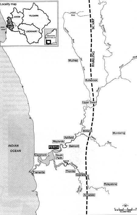
The Swan estuary is located in the central part of the Swan coastal plain in the southwest of Western Australia at 31o45'S, and 116o04'E. The Swan River is the continuation of the Avon River as it flows into the coastal plain from the Darling plateau, passing down an escarpment called the Darling Range. The estuarine section of the river extends over 53 km. It has a shallow tidal river, a broad basin and a narrow inlet channel, which joins the Indian Ocean. Several freshwater tributaries enter the estuary, the major ones being Canning River, Helena River and Ellen Brook, each of these are fed by several streams (Fig. 1). The Avon River is about 300 km long and before it becomes the Swan River, is joined by several tributaries, winding through vast areas of agriculture, native forest and semi-arid zones with several salt lakes. The catchment area of the Swan-Avon river system is over 190,000 km2. The dominant feature of the catchment area is agricultural development with sheep and cattle farming and wheat cultivation. It is estimated that 75% of the Avon River catchment has been cleared for agricultural purposes since European settlement.
The Swan coastal plain enjoys a Mediterranean climate characterized by cool and rainy winters and warm to hot summers. The average annual rainfall is between 800 and 900 mm, the rainfall decreasing from west to east. The winter water temperature ranges from 10 to 14oC and the summers 22-30oC (Fig. 2).
|
| Fig. 1 The catchment area of the Swan-Canning River System (courtesy of the Swan River Trust 1996). The sampling sites of the project were located on the urban catchments of Swan and Canning River systems and the tributaries – Helena River and Ellen Brook and many streams and drains joining the system. |
| (original size image) |
 |
| Fig. 2. Rainfall and mean volume of flow in the Swan-Canning system (courtesy of Swan River Trust 1999). |
The Swan River estuary is characterized by extreme seasonability in freshwater flow and salinity. There is a salinity gradient from the lower to the upper estuary for much of the year. During summer and autumn, the gradient is well established with the mouth of the estuary at seawater salinity, and progressively decreasing salinity towards the headwaters (Hodgkin 1987). The rains during winter to spring flush the river, lowering the salinity of the surface water of the upper estuary to often less than 3 ppt. In the same period, the salinity of the surface water in the lower estuary may range from 3 ppt in a wet year to 20 ppt in a dry year. The winter fresh water flow may result in the vertical stratification of the lower estuary with the saline water at the bottom and the fresh water at the surface. This vertical stratification is less evident towards the head of the estuary. At the end of spring, the fresh water runoff slows down and the saline water of marine origin moves upstream. With the penetration of this wedge of salt water, the fresh water mixes with the deeper saline water aided by wind, and summer conditions are re-established. The duration, timing and intensity of winter rains and the dry summer period determine not only the salinity profile of the river but also the nutrient status, the biota, and the ecology of the river (Fig. 3).
Like other estuaries, the Swan is a meeting place where the fresh water from the catchment and the saline water from the sea meet. It is a highly productive place. There are 137 species of fish belonging to 70 families recorded from the Swan River estuary. It is estimated that more than 300 tons of fish are caught annually by commercial fishermen from the Swan River estuary. The magnitude of the recreational fishery is estimated to be equal to that of the commercial fishing (Loneragan et al. 1987).
 |
| Fig. 3: Salinity changes in the Swan River in summer and winter (John 1994). |
More species of water birds have been recorded at the estuary than at any other wetland in south Western Australia. Now the river is the most important aquatic recreational resource of the community. With an active yacht club, at least 25,000 registered vessels use the river at some time of the year. The use of the River for private pleasure craft covers yacht clubs, private marinas, vessels on permanent moorings, water skiing, speed boat courses, rowing and swimming. In addition to pleasure activities, the River still serves as a source of public transport within the city as well as to a neighbouring island. Commercial pleasure cruises also use the River (Spencer 1987).
Eutrophication is a severe problem afflicting the health of several estuaries in Western Australia (Swan River Trust 1999). The Swan River estuary is now beginning to show symptoms of eutrophication. Nutrient and algal studies indicate that the Swan can be classified as mesotrophic to eutrophic. The nitrate and phosphate levels are at times very high. Nitrate level may peak up to 3000 µg 1-1 and phosphates up to 300 µg 1-1; the highest levels are recorded during the winter. There is a very high correlation between nitrogen and phosphorus levels and the rainfall (John 1987; 1994).
The chlorophyll a biomass of the upper reaches of the Swan may reach up to 250-300 µg 1-1 during the spring algal blooms. As the winter rains bring large quantities of nutrients into the river, spring blooms are initiated in the lower and upper reaches by different species of phytoplankton. The lower reaches of the Swan respond to the nutrient enrichment during the winter by initiating diatom blooms. Skeletonema costatum - a well-known phytoplankton of enriched coastal waters in many parts of the world, is the dominant plankton in the estuary. During spring, phytoflagellate blooms are common in the estuary; it is the green alga, Chlamydomonas globosa that causes blooms in the upper estuary (John 1987; 1994).
The nutrient levels are much higher in the upper estuary than those at the lower estuary. The shallow upper estuary also experiences more planktonic blooms with chlorophyll a levels up to 300 µg 1-1. The lower estuary is better flushed with sea water with less number of drains from the catchment. During April 1991, a species of Gymnodinium, a tiny dinoflagellate, caused a massive bloom with density up to 1.5 million cells m1-1 in the upper estuary. The prolonged occurrence of this bloom with a distinct discolouration for several weeks caused considerable alarm among the public (Swan River Trust 1991). Occasionally, there are reported cases of minor patchy blooms of the cyanobacteria Microcystis and Anabaena in the upper reaches of the Swan River. This is often the result of overflow from eutrophic lakes nearby and is of a temporary nature. In February 2000, after a high rainfall, a bloom of Microcystis aeruginosa form flos. aquae occurred, although confined to the edges of the river and lasted for two weeks, resulting in the closure of the estuary to the public.
Thus unusual patterns of rainfall can trigger some of these blooms. Unusual rains in summer or autumn can trigger dinoflagellate blooms (e.g. Scrippsiella) as they bring in the extra nutrients and the appropriate nitrogen to phosphorus ration to initiate the blooms. There has also been massive growth of macroalgae such as Enteromorpha and Rhizoclonium in the shallow mid-estuary.
The hydrology of the river is linked to its potential eutrophication. The link between high chlorophyll a biomass and phosphorus and nitrogen loading is well established in the Swan River. Though some of the nutrients are flushed into the sea, a considerable amount is cycled through the biota, thereby enhancing productivity and enriching the sediment. The sediment therefore becomes a continuous source for nutrient release especially under deoxygenated conditions created by the unusual rainfall. As the annual load of nutrients increases, the sediment source of nutrients also increases, but the flushing rate does not increase correspondingly. A trend in a shift from frequent diatom blooms to phytoflagellate blooms, especially the dinoflagellates, has been observed in the summer-autumn period in recent years, and is an obvious sign of increasing nutrient loading to the estuary. The nutrient loading by drains and streams after unusual rains in summer-autumn exacerbate the frequency of blooms.
Streams from the catchment areas carry large amounts of phosphorus and nitrogen to the Swan River. Most of the phosphate (80-90%) comes from the Avon River and its tributaries, Ellen Brook, Southern River and Jane Brook, and from urban drainage such as the King William Street drain. The amount of phosphorus loading for each square meter of the estuary is estimated to be 1.8 to 2.4 g. The input of nitrogen and phosphorus depends upon the type of soil of the catchment and the land use. Cultivated lands contribute more phosphorus than lands with native vegetation. Hilly rural areas contribute less nutrients than cultivated plains. Avon River with its 120,000 km2 catchment area contributes the highest amount of nutrients into the Swan River. However, the nitrogen to phosphorus ratio of the input is high, i.e., more nitrogen is discharged and more phosphorus is retained in the catchment. This is due to the nature of the soil. The laterite soil of the catchment tends to retain phosphate. Most of the area of Avon River catchment is used for dryland agriculture. This area generates 18% of the total Western Australian agricultural income. The farmers traditionally have used high amounts of fertilizers. During the rainy season, the Avon River flows, but during the dry summer months, it dries up, leaving a chain of disconnected, tree-lined pools. The incidence of serious flooding in the Avon is once in every 10 years. In an attempt to prevent flooding of the towns, the government introduced the Avon River Training Scheme between 1956 and 1973 by mechanically clearing the sediment and vegetation from the water channel. While it has prevented flooding, it has also resulted in increased flow, which increased input of nutrients into the Swan and increased erosion and siltation (Seal 1991). The pattern of rainfall, type of land use and soil are important in determining the ratio of nitrogen to phosphorus in runoff (Table 1).
| Table 1. Average nutrient input into the Swan River (1987-1991); examples of the main sources. | ||||||
| Source | Mean rainfall (mm) | Catchment area (km2) | Total N (tonnes) | Total P (tonnes) | N:P ratio | |
| (AR) | Avon River | 700 | 120,000 | 270 | 17 | 15.50 |
| (CB) | Ellen Brook | 719 | 700 | 70 | 25 | 2.74 |
| (CMD) | Claisebrook Main Drain | 823 | 16 | 10 | 1 | 10.00 |
| AR = rural diffuse source characterized by dry agricultural lands, laterite soils and natural vegetation, CB = rural point sources with sheep farms and piggeries, CMD = urban diffuse source (Data, courtesy of Deeley, 1992, Water and Rivers Commission, Perth). | ||||||
The pattern of rainfall and soil wetness is important in rural catchments. Total nitrogen input from the Avon catchment area is very large. The highest amount of phosphorus loading comes from animal farms, particularly piggeries among the rural point sources. For example, Ellen Brook catchment, a rural area with many piggeries and sheep farms, contributes 25 tonnes of phosphorus to the Swan River as opposed to 70 tonnes of nitrogen. This type of nutrient loading with a low nitrogen to phosphorus ratio is more conducive to blue-green and dinoflagellate blooms as the primary productivity of the upper estuary is limited by nitrogen. Rural point sources commonly have very high levels of soluble phosphorus. For example, 60-70% of the total phosphorus load for Ellen Brook is in soluble form, readily taken up by phytoplankton (Deeley, 1992).
Urban catchments have a very efficient drainage network. Surface runoff is high in urban areas. Input from urban catchments has high particulate loading; nitrogen and phosphorus loads are significant throughout the year and nutrient export rates are similar to broadcare rural land uses. With the increase in population of Perth, currently 1.4 million, the nutrient input into the river from urban development can only increase. River front residences are in high demand. The pattern of colonization of Western Australia clearly shows the high demand for areas closer to the river. With the lavish supply of fertilizers to the foreshore gardens, the nutrient input into the river continues to rise.
During summer, the salt wedge from the lower estuary moves up. This is followed by marine diatom blooms moving up. This pattern is broken by sudden input of freshwater discharge with high amounts of nitrogen and phosphorus. The salt water is isolated; the sudden discharge of enriched water makes high demand upon oxygen. Diatoms (the normal dominant phytoplankton component) are replaced by phytoflagellates or cyanobacteria; the fish die locked in salt water without sufficient oxygen. In February 1992, a fish kill of this type occurred in the Swan River.
In addition to surface water flow, ground water contributes at times substantially to the nutrient loading of the Swan River estuary. High flows of nutrient rich ground water have been identified at several locations along the Swan River. It is estimated that ground water contribution to the nutrients of the river is close to 16% of the total nutrients entering the river through surface water flow. There are localised inputs of nutrients along the margin of the Swan River. This may be of vital importance in triggering algal blooms in summer (Swan River Trust 1999).
The flow of the tributaries of the Swan River has been significantly altered in summer due to dams built in the past. Canning Dam and Kent Street Weir and unauthorised damming and diversion for irrigation all have altered the flow and ecology of the system. Impounded freshwater pools, replacing flowing tributaries have contributed to toxic cyanobacterial blooms (Anabaena spp.) which occurred in the Canning River in 1994, 1996 and 1998.
Diffuse pollution rather than point sources, continue to contribute to the nutrient enrichment of the estuary. Garden fertilizers and septic tank leaching from the urbanised land reach the estuary through urban drains and groundwater. It is estimated that 40 kg of total phosphorus per hectare annually is used for urban gardens. This is more than double the application rate in agriculture areas. Over 500 tonnes of fertilizer is used in the Perth metropolitan area every year. Park and turf irrigation practices further add to the problem. Clearing remnant vegetation in urban areas for housing and development cause erosion which results in sedimentation and nutrient enrichment in the river.
Dewatering may be required for urban buildings, including tunnels. Polluted water may have to be discharged into storm water drains and the river. Very recently a tunnel (1.6 km) was built to link the northern part of the city to the Swan River, which required dewatering.
Although point sources such as industrial and commercial sources of pollutants in the Perth metropolitan area have been minimised by legislation since the 1950s, hard surfaces (paved areas, roads (concrete, bitumen) etc) generated by urban commercial and industrial developments have enhanced runoff to the water courses (Fig. 4).
River foreshores have been used in the past as waste disposal sites, landfills and rubbish tips. Although these have been closed, they do pose a problem, when disturbed for new development. Mobilization of nutrients and contaminants may leach into the river or may be carried to the river by ground water (Fig. 5).
It is estimated that there are 200-300 km of urban drains managed by the Water Corporation of Western Australia and 2,500 km of surface and subsurface drains under the control of the local government. They virtually convert non-point sources into point sources by discharging into the Swan River. Several drainage systems in the metropolitan area are known to contribute substantially to the nutrient loading of the Swan River estuary (Fig. 6).
 |
| Fig. 4. Industrial areas of the Swan-Canning System (courtesy of the Swan River Trust 1999) |
 |
| Fig. 5 Landfill wastes disposal sites (courtesy of the Swan River Trust 1999). |
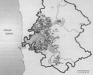 |
| Fig. 6. Sewered areas and Water Corporation drains within the Swan-Canning system (courtesy of the Swan River Trust 1999). |
The design of sampling for the current project required large numbers of sites – reference (Pristine) and monitoring sites, representing all different types of drains and streams, both natural and man made. In order to develop a predictive model and a classification system, the whole urban catchment area around the Swan-Canning River estuary had to be covered. While selection of monitoring sites (impacted sites) was relatively easy, selecting reference sites was difficult. The historical data on water quality and catchment characteristics kept by the Water Corporation of Western Australia, Water and Rivers Commission and local government agencies were examined (Atkins & Klemm 1987; Swan River Trust 1994; 1996; Henderson 1995). Nutrient loading by urban drains and streams to the Swan-Canning River was monitored by the Swan River Trust from 1987 – 1992 on a sporadic basis, involving 15 major tributaries including artificial drains. The streams and drains monitored by the Swan River Trust included rural and urban sub-catchments (Swan River Trust 1994). The Water Authority of WA (now Water Corporation of WA) had compiled data on 104 sampling sites from 59 drains discharging into the Swan-Canning, 11 drains into the lakes and wetlands and 14 main drains discharging into coastal waters, some of these data go back to 1968.
The catchments from which the sampling sites were selected belong to five zones based on land use (Fig. 7): Ellen Brook, Hills, Urban North, Urban South and Canning. After visiting several sites, and considering the land use and stream characteristics such as peripheral vegetation, bank stability etc. the features that affect the ecological integrity of the system, a final selection of 200 sampling sites was made. These sites represent the 31 sub-catchments recognised in the urban rural (semirural) area around Perth (Fig. 8).
In general, the reference sites had relatively lower nutrients, better peripheral vegetation and lower pH and lower electrical conductivity than the monitoring sites (impacted). Considering the historical development of Perth, the current land use and nutrient status, most of the impacted sites were proximal to the Swan-Canning estuary. Most of the reference sites were from suburban and semirural sites in hills and Ellen Brook Catchment away from the urban development, where the remnant native vegetation is less disturbed. The replacement of indigenous sclerophyllous plants by soft leaved exotic plants in the urban areas obviously had an impact on organic loads in the river.
 |
| Fig. 7. Urban catchments of the Swan River system (courtesy of the Swan River Trust 1996). |
The Canning catchment includes a large Botanical Park (Araleun Botanic Park) bush lands suburban town, bush lands, housing development and hobby farms and Yule Brook, Bickley Brook, Ellis Brook, Southern River, Wungong River and Bannister Creek and Littoria Main drain covering an area of 511 km2. Southern River and Wungong River contribute high amounts of phosphorus to the Canning River. The Ellen Brook Catchment area is the largest with 715 km2 and is an important feeding tributary to the Swan River estuary. This catchment contributes the highest amount of phosphorus to the Swan River.
|
| Fig. 8. Catchments of the Swan-Canning system on the coastal plain (courtesy of the Swan River Trust 1999). |
Many natural streams in this catchment have been modified for drainage purposes and are privately owned. Chicken, pig and cattle farms in this catchment continue to provide high phosphorus loading to the river. The hill catchment covers an area of 420 km2 with Helena River, Blackadder Creek, Jane Brook, Susannah Brook and Millendon. Land use here is low density housing and hobby farms. Most of the relatively undisturbed sites are located in this catchment.
The northern catchment (area 257 km2) comprises Claisebrook Main Drain, Bayswater Main Drain, Bennett Brook, St Leonards Creek and Henley Brook. High concentrations of nitrogen are loaded into the river through these streams. The northern urban catchment has been undergoing rapid growth and development over the past 20 years. The south urban catchment comprises Perth Airport Drain, Belmont Drain, Mill Street Main Drain, South Perth Drains etc (202 km2) and again delivers high concentration of nutrients both nitrogen and phosphorus into the system. The majority of the impacted sites are from the urban catchments close to the river.
Virtually all the catchments have been affected, some more severely than others, by human impact since European settlement and therefore the so called 'reference sites' can only be described as 'relatively less impacted or relatively pristine'. However, Perth urban and rural catchments do provide us with a variety of streams and drains under varying degree of habitat characteristics and degradation, suitable for developing a predictive model for biomonitoring.
The geographic location of each site was recorded using a Magellan GPS 2000 satellite navigational instrument during the second sampling. The site positions were recorded as degrees latitude/longitude. The individual site distance from the Swan/Canning Estuary, soil type and water table depth were extrapolated from the Perth UBD (1995) and the Perth Groundwater Atlas (WRC 1997).
A total of 200 stream sites were originally selected and surveyed for this study between August 1996 and December 1996. Each of these sites was numbered in a logbook with codes "Urban 1-200". The study sites represent 31 subcatchments of the Swan, Canning River system (Fig. 8). A number of sites were selected from 10 subcatchments known historically to have "low" nutrient concentrations, based on ANZECC guidelines (ANZECC 1992;1999, SRT 1997), these include the Avon River, Helena River, Jane Brook, Upper Canning, St Leonard's Creek, Ellis Brook, Bickley Brook, Neerigan Brook, Upper Woodlupine and Upper Wungong Brook. The rest of the sites were selected from 17 subcatchments known to have "high" levels of nutrients (SRT, 1997), which include Ellen Brook, Millendon, Blackadder Creek, Belmont Main Drain, Mills Street Main Drain, Yule Brook, Southern River, Lower Wungong, Bannister Creek, Lower Canning, Bullcreek, Claisebrook, Maylands, Bayswater Main Drain, Bennett Brook, Upper Swan, and Henley Brook. The majority of "low nutrient" sites tend to be located close to the Darling Escarpment in the eastern zone of the study area with minimal land disturbance. The majority of "high nutrient" sites tend to be located closer to the Swan Canning Estuary in the west with relatively heavy land disturbance. Out of 200 sites, 182 sites were surveyed in autumn-winter 1997 and 165 study sites in spring-summer 1997. Each study site was photographed and a data set with a brief description of all sites was created. A random assortment of eight sites with photographs and brief descriptions is presented in Appendix 1.
Indices with arbitrary ranges were used to classify stream conditions (Table 2). The state of the riparian vegetation was examined 10-20m from the shoreline and classified on the basis of a) degradation and loss of canopy cover and b) proportion of riparian plants that are native. Using maps the distance from the Swan/Canning Estuary for each site was calculated, as was water table depth and groundwater salinity. The soil type and surrounding land use were classified into categories allocated to each site. The clarity, odour and surface appearance of stream water was assigned a numerical category based on visual observations. The dominant substrate algae, planktonic algae, submerged macrophytes, emergent macrophytes and floating macrophytes were observed for each site and were ranked based on arbitrary relative abundance. The assessment methods of the stream catchments in the Perth metropolitan are modified from techniques used by Mitchell (1990), Jarlman et al. (1996) and John (1998).
The pH of the water was recorded using a Beckman hand held pH meter. Electrical conductivity was measured using a Hanna Instruments 4I 8733 conductivity meter. A WTW Dissolved Oxygen meter was used to measure both the temperature and the oxygen content of the water. Flow was measured with a General Oceanics flow meter. The width and depth of the site of streams or drains were recorded using a tape measure for each sampling. The riparian vegetation, sediment characteristics and surrounding land use were also recorded.
Water samples collected in 750 ml plastic sample bottles were kept on ice and taken to the Algology laboratory at Curtin University, Perth, Western Australia. Variables tested were; colour, alkalinity, turbidity, NH3-N, NO3-N, Total N, Total P, Filterable Reactive P and pigments (Chlorophylls a, b and c, and phaeophytin). The samples were sent for chemical analysis to Analabs Pty. Ltd. where the parameters were analysed according to standard methods (APHA 1995).
An artificial substrate sampler designed by John (John 1998) known as the JJ Periphytometer (Fig. 9) was used for uniform collection of diatom samples. Ten glass slides were placed in each sampler, and 10 lb fishing line was threaded through the holes in the sampler. The sampler was then suspended in the water, with the fishing line attaching the sampler to a convenient, sturdy point, such as a bridge strut, pipe or tree branch. The sampler and attachment line was camouflaged as best as possible, before being retrieved on a subsequent visit after two weeks to each site. Of the total of 200 sites initially selected, 16 subsequently dried out and were abandoned. One JJ Periphytometer was suspended in each of the remaining sites, a total of 184 periphytometers were submerged for a duration 14 days in 1997. Vandalism and loss (due to flash floods, or exposure from dropping water levels) of periphytometers, further reduced the number of sites available for biomonitoring. A total of 148 samplers were recovered for the Autumn/Winter sampling (April-June) 1997 and 146 for the Spring/Summer sampling (October-December) 1997 representing a 20% loss rate for both sampling seasons. A duration of 14 days was found to be sufficient for a stable climax community to be reached on glass slides.
Periphyton scraped from 5 glass slides was transferred into 25 ml plastic screw capped vials containing equal volumes of Lugols solution (distilled water plus 2-3 drops of Lugols Iodine). The specimens stored in Lugols were useful only for short term analysis and cell count.
 |
| Fig. 9. JJ Periphytometer – an artificial substrate collector designed by J John. |
Samples were counted on a Sedgwick Rafter cell counter (S50). The samples were mixed thoroughly to break up algal flocs and suspend cells, 1 ml aliquots were pippetted onto the counting grid of the Rafter counter. Micro-algal counts were conducted at a magnification of 400 X using a Olympus binocular compound microscope, individual fields of view were scanned. The number of cells were then divided by the number of grid squares used (each square = 1 ml) to calculate number of cells/ml. To derive periphyton cell density (cells/cm2 glass) the initial count was multiplied by the number of millilitres of liquid in which the scrapings were stored giving the total number of cells from the 5 glass slides. This number of cells was divided by 5 (number of slides) and finally divided by the surface area of each slide (2.54 cm ´ 7.62 cm ´ 2).
Periphyton scraped from 5 glass slides (from the JJ Periphytometer) were transferred to 25 ml plastic screw cap vials containing equal volumes of Transeau's Algal Preservative. Preparation of diatoms was conducted using standard techniques for obtaining clean diatom frustules from samples (John 1983).
The preserved periphyton was mixed well to break up attached diatoms and to suspend the algae. Approximately 10 ml of this mixed sample was transferred into an acid washed 100 ml Pyrex Beaker. To each beaker, an equal volume (10-15 ml) of concentrated (90 %) Nitric Acid was added. The beakers were placed on a hot plate and allowed to boil and evaporate within a fume cupboard. Occasionally some of the samples with high organic content reacted violently with acid. To prevent excess spluttering of acid, deionised water was added (1 ml at a time). After boiling, the suspension was allowed to cool. They were transferred to labelled plastic centrifuge tubes and topped up with deionised water. The samples were then centrifuged at 3500 rpm for 5 minutes, after which the supernatent was pippetted out with the pellet of diatom frustules remaining at the bottom. After this the pellet was re-suspended in deionised water. This process was repeated a few times to ensure all trace of the nitric acid was removed. The 'cleaned' diatom frustule material was then stored for making permanent slides.
Some of the samples were observed to be relatively dense with frustules, these were diluted further and observed under a phase contrast microscope. Once the frustules under the coverslip did not overlap each other then that dilution factor was used for preparing a permanent slide. In most samples 1:1-1:3 (sample water) was sufficient to dilute the samples, in some cases up to 1:9 was necessary for dense samples. Approximately 1 ml of the 'cleaned' sample was pippetted onto clean glass coverslips (22 mm x 22 mm). The coverslips were placed onto a hot plate at low temperature (60o C) and the solution allowed to slowly evaporate. It was necessary to ensure even distribution of the suspension on the coverslip and the sample was further mixed using a micro pippette to draw up and dispense the sample back onto the coverslip to ensure even dispersal of frustules. Once dry, the coverslips were placed onto clean glass slides to which a drop of naphthrax mounting medium (soluble in Toluene) (Refractive Index 1.7) had been added. The slides were heated on a hot plate until all the toluene evaporated, leaving the naphthrax. Once free of bubbling, the slide was removed from the hotplate and allowed to cool and harden at room temperature. Three replicate slides were made from each sample to ensure maximum representation from the 'cleaned' sample. All slides of diatoms have been labelled and deposited with the Curtin University Diatom Herbarium, School of Environmental Biology as 'voucher slides' for future reference.
Diatoms are identified to the species level, based on their unique, stable, morphological characteristics observed using oil immersion microscopy. In this study diatoms were identified, to species level, using standard Australian diatom literature and the vast collection of diatom literature and atlases at the International Diatom Herbarium, Curtin University: John (1983;1998), Thomas 1983, Foged (1978) and Holland & Clark (1989). Nomenclatural confirmation was made using Round, Crawford & Mann (1990), Metzeltin & Witkowski (1996), Metzeltin & Lange-Bertalot (1998), Krammer & Lange-Bertalot (1986), Lange-Bertalot (1996), Lange-Bertalot & Metzeltin (1996) and Patrick & Reimer (1966;1975).
The permanent slides of diatom was scanned first under 100 X, then 400 X to assess a general profile of the frustules and then examined under 1000 X oil immersion and frustules counted scanning the slide from top to bottom. Frustule count ranged from 100 – 400 depending upon the density of frustules (two vales were counted as one frustule). Count up to 400 was found to be adequate to include all species on the slide according to initial trials conducted. The relative frequency of each species was calculated using a scoring sheet with all the species names.
The diatoms were photographed mostly under oil immersion (1000 X) using a Vanox photomicroscope. The Iconographs with the identification and an introduction to the Biology and Ecology of diatoms are presented in a separate volume (A Guide to Diatoms as Indicators of Urban Stream Health).
| Table 2. Environmental variables. | |||
|---|---|---|---|
| Riparian Damage: (RD) | 1 | = | Intact, stable plant riparian community, high canopy cover. |
| 2-4 | = | Increasingly damaged riparian community, reduced canopy cover | |
| 5 | = | Stream banks only occupied by grasses, no canopy cover | |
| % Native Vegetation: (nV) | 1 | = | 0-20% of Stream Catchment vegetation are native species. |
| 2 | = | 20-40% | |
| 3 | = | 40-60% | |
| 4 | = | 60-80% | |
| 5 | = | 80-100% | |
| Water Table Depth: (WTD) | 1 | = | Water table 1-2 metres below surface |
| 2 | = | 2-3 metres | |
| 3 | = | 3-4 metres | |
| 4 | = | 4-5 metres | |
| 5 | = | >5 metres below surface | |
| Ground Water Salinity: (GWS) | 1 | = | <250 mg/L TDS |
| 2 | = | 250-500 mg/L TDS | |
| 3 | = | 500-1000 mg/L TDS | |
| 4 | = | 1000-1500 mg/L TDS | |
| 5 | = | >1500 mg/L TDS | |
| Stream Soil Type: (ST) | 1 | = | Red clay loam/gravel |
| 2 | = | Clay/silt/mud | |
| 3 | = | White Sand | |
| Catchment Land Use: Intensity (CLU) | 1 | = | Mainly natural forest, some urban settlements and hobby farms 0-20% catchment cleared for use. |
| 2 | = | Urban settlement, some remnant native species in parks 20-40% of catchment cleared for use. | |
| 3 | = | A significant area of land used for urban housing, horticulture and agriculture 40-60% of catchment cleared for use. | |
| 4 | = | A significant area of land used for urban housing and light industries, 60-80% of catchment cleared for use. | |
| 5 | = | Industrial Park, 80-100% of catchment cleared for use | |
| Distance from Estuary (DE) | ||||
| Visibility of Water: | 1 = Clear, | 2 = Good, | 3 = Fair, | 4 = Poor |
| Odour: | 1 = None, | 2 =Effluent, | 3 = Anoxic, | 4 = Algal |
| Foaming: | 1 = None, | 2 = Detergent, | 3 = Surface spots | 4 = Scum |
| Substrate Algae: | 1 = Not visible, | 2 = Thin film, sporadically distributed, | 3 = Thick mat, widely distributed | |
| Planktonic Algae: | 1 = Not evident, | 2 = present in water column, | 3 = Forms bloom in water | |
| Emergent Plants: | 1 = None, | 2 = Low, | 3 = Medium, | 4 = High (growing right across stream) |
| Submerged Plants: | 1 = None, | 2 = Low, | 3 = Medium, | 4 = High (covers entire stream bed) |
| Floating Plants: | 1 = None, | 2 = Low, | 3 = Medium, | 4 = High (covers entire stream surface) |
Data were collated and entered into MS Excel spreadsheets: fresh cell count, physico-chemical data, environmental variables, species list, and relative abundance of species in each site.
Fresh cell counts from each sampling period were correlated with pH, electrical conductivity, total nitrogen, total phosphorus and riparian degradation and all other environmental variables.
Classification of the sites based on environmental variables and diatom species distribution was performed separately using the multivariate pattern analysis software package PATN (Belbin 1993). Sites with a completed set of seven environmental variables were finally used for classification. Values of each variable were standardised (range standardisation) using option 4 in the TRND module of PATN. Association analysis was performed with the module ASO using the Bay-Curtis measure.
Classification of 146 sites in summer 1997 according to environmental variables was performed using the multivariate analysis package PATN. Only sites with a complete set of seven environment variables were used to perform the classification. These were Alkalinity, NH3, TKN, TN,SRP, TP and colour. Values of each variable were standardised (range standardisation) using option 4 in the TRND module of PATN. Association analysis was performed with the module ASO using the Bray-Curtis measure. Clustering of all the sites was then done by using an Agglomerative Hierarchical Fusion method using flexible unweighted pair group mean averages (UPGMA). Output was then generated and visualized using the DEND and GDEF modules.
Taxa with frequency scores > 1% were present in at least 5% of sites selected for classification. Data were log 10 (n+1) transformed prior to Association analysis with Bray-Curtis measure. Clustering of all sites was performed by an Agglomerative Hierarchal Fusion method by using flexible unweighted pair group mean averages (UPGMA). Output was then generated and visualized using the DEND and GDEF modules. The full data sets are presented in Appendix 2 and 2a.
Patterns in the environmental data were explored using Principal Components Analysis (PCA). The multivariate analysis package PC-ORD V3 was utilized to perform the analysis and generate graphical output and printed diagnostics. A standardization was performed on the values for each variable using the formula Xij/((sumXj**p)**1/p. Using p = 2 is the Euclidean equivalent of relativization of column (variable) totals. The double asterisk is used to signify an exponent.
The relative contributions of the diatom species was also determined by Principal Axis Correlation. The Biplot for the SSH ordination of all sites with vectors for diatom species with a correlation coefficient of < 0.4 was generated. Significance for each correlation coefficient was tested by MONTE CARLO procedure using at least 499 random simulations for each species.
In an attempt to identify characteristic species of each group, a species list of diatoms common at least to 40% of sites in each group was ordered by declining frequency of occurrence.
Multidimensional Scaling MDS (semi strong hybrid MDS Belbin 1993) was used as the ordination method. This was done both with the diatom species and environmental factors. This program is contained within the PATN software package (Belbin 1993). SSH is considered to be the most robust ordination method available. It is able to cope with the typical situation in which the response of taxa to underlying gradients are unimodal, noisy and skewed (Marchant et al 1994).
The environmental measures were correlated with the ordination. The environmental factors were correlated with the ordinations by using the Principal Axis Correlation (PCC) routine in PATN. The procedure calculates a vector of maximum linear correlation for each environmental variable in the reduced dimensional space. PCC also specifies the direction taken by a vector which can then be plotted to represent the trend in relation to the environmental variable on the ordination (also called a biplot). Significance levels for each correlation coefficients were tested by MONTE CARLO procedures; 499 simulations of randomised environmental data were used in all analyses. This was also done on the diatom data.
The state of the 'health' of the urban streams was analysed by the distribution pattern of indicator species generated by classification superimposed on the group classification of environmental variables of the sites.
The classification of sites on the basis of diatom distribution was imposed on the environmental data. This was to see how far the environmental data can predict the group membership in the classification by diatom distribution.
A hierarchical classification of species was also performed to provide ordering of the species for a two way table of the data matrix. Clustering the species also provides insight into which species tend to occur together and which do not (Belbin 1993). This is one of the most useful ways of displaying the results of a classification. It imposes the dendrogram ordering, with the defined groups back on the data matrix itself. The site groups can be analysed on the basis of species composition while species groups can be analysed by location at sites. The data matrix was transposed and then analysis of the log transformed species frequencies was performed using the two step association.
An attempt was made to derive an index, which would indicate whether a site could be classified as a reference or monitoring site based on the diatoms.
Using the two-way classification (PATN analysis) of the diatom abundance, the sites were segregated and the indicator species of reference sites were identified. The group classification obtained from the diatom data set was then used in a discriminant function analysis of the environmental variables which were highly correlated to the Multidimensional Scaling ordination (Alk, GWS, CLU, RD, CS, Colour, nV, WTD). The probability of a site being correctly classified by this method was then obtained. This is similar to the method used by Wright (1995) for obtaining site classification probabilities. Discriminant function analysis was performed with the software program SPSS 7.1.
The probability of occurrence (P) of species i was then calculated as:
Pi = g = 1nS QgRgi
where Qg is the probability that the site is a reference site as determined by the environmentally derived discriminant functions and Rgi is the proportion of sites in which the species was recorded.
Using this formula an index was derived using the ratio of the sum of the combined probabilites of the reference indicator species (27 species) multiplied by their abundance + 0.1 (to account for the possibility of the total absence of species as division by zero is not valid) divided by the sum of the combined probabilites of the unexpected species (30 species) + 0.1 (to account for the possibility of the total absence of species as division by zero is not valid).
The diatom index is I =
(Pr * Ar) + 1
(Pu * Au) + 1
where:
A = abundance of r(reference) or u(unexpected) species
P = probability of r(reference) or u(unexpected) species
This index was tested on data collected on every site in spring-summer 1997 and further tested on 11 randomly selected sites from the autumn-winter sampling of diatoms. A copy of the spreadsheet in which values of species present can be tested against the complete data set by deriving the probabilities is presented in Appendix 3.
Positive correlation has been found between fresh cell density, total phosphorus, total nitrogen and colour (Figs. 10, 11 and 12) as well as Riparian damage. Multiple comparisons of mean habitat characteristics and periphyton density as obtained by cell count from the periphytometer, with significant levels are shown in Table 3. The results relate to periphyton count of samples of summer 1996. Similar trends were observed in samples collected in 1997. Some of the sites originally classified as reference had to be reclassified as 'intermediate' based upon correlation.
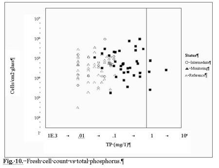 |
| Fig. 10. Fresh cell count vs total phosphorus. |
| (original size image) |
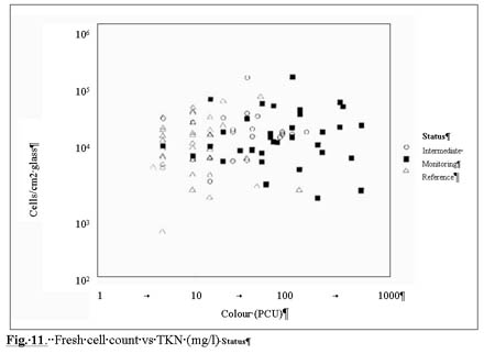 |
| Fig. 11 Fresh cell count vs TKN (mg/l) Status |
| (original size image) |
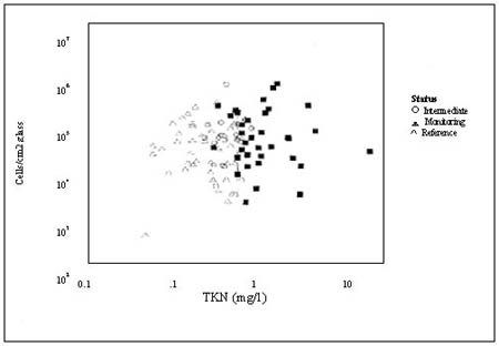 |
| Fig. 12. Fresh cell count vs colour (PCU). |
| (original size image) |
Site Classification Based on Environmental Variables
Hierarchical classification of sites with the addition of prior nomination of reference or monitoring rating, is presented in Fig. 13 (the dendrogram refers to 1997 summer collection of 146 sites). The classification generated 12 groups (Table 4). Groups 4 and 9 to 12 comprised most of the reference sites with more than 95% in each group. Groups 1, 6 and 8 had more than 60% of sites classified as monitoring. Groups 9 to 12 were predominantly located in the hills area or away from the urban catchments, while groups 6 and 8 were in either industrial or heavily impacted agricultural areas.
| Table 3. Pairs of variables with strong correlations (r > 0.45). | |
|---|---|
| Variable Pairs | r Value |
| Colour – SRP | 0.74 |
| TKN – TN | 0.97 |
| TKN – TP | 0.94 |
| TN – TP | 0.91 |
| Cells / cm2 - % Diatoms / Non Diatoms | -0.46 |
| Table 4. Composition of final grouping of sites according to classification based on environmental parameters. | |||||
|---|---|---|---|---|---|
| Group | Reference | % | Monitoring | % | Total |
| 1 | 2 | 12.5 | 14 | 87.5 | 16 |
| 2 | 0 | 0 | 2 | 100 | 2 |
| 3 | 1 | 33 | 2 | 66 | 3 |
| 4 | 1 | 100 | 0 | 0 | 1 |
| 5 | 2 | 66 | 1 | 33 | 3 |
| 6 | 10 | 37 | 17 | 63 | 27 |
| 7 | 1 | 25 | 3 | 75 | 4 |
| 8 | 10 | 34.5 | 19 | 65.5 | 29 |
| 9 | 19 | 100 | 0 | 0 | 19 |
| 10 | 6 | 100 | 0 | 0 | 6 |
| 11 | 34 | 97.1 | 1 | 2.9 | 35 |
| 12 | 1 | 100 | 0 | 0 | 1 |
| Fig. 13. Dendrogram for the hierarchical clustering of the 146 sites, using UPGMA linkage of Bray-Curtis similarities of the range standardized environmental data. (Enlarged Figures) |
 |
 |
 |
Ordination of Environmental Variables
Superimposing the site classification on the principal component analysis results in the segregation of the reference and monitoring sites (Fig. 14). Correlation matrix of the seven environmental variables is presented in Table 5. There is positive correlation between the ordination scores of axis one and the magnitude of the variables, TKN,TN and TP. These three variables increased linearly from low values in reference sites to mixed sites and elevated values in the monitoring sites (Table 6).
| Table 5. Correlation matrix of the seven environmental variables. | |||||||
|---|---|---|---|---|---|---|---|
| Alk | Colour | TKN | TN | NH3 | TP | SRP | |
| Alk | 1 | ||||||
| Colour | 0.1462 | 1 | |||||
| TKN | 0.03647 | 0.1726 | 1 | ||||
| TN | 0.03353 | 0.1721 | 0.9662 | 1 | |||
| NH3 | 0.4845 | -0.03398 | 0.07296 | 0.0681 | 1 | ||
| TP | -0.01289 | 0.2358 | 0.6842 | 0.6651 | 0.1843 | 1 | |
| SRP | -0.005297 | 0.6983 | 0.1675 | 0.1753 | -0.000756 | 0.3074 | 1 |
| A correlation matrix of the environmental factors showed there was positive correlation between TKN, TN and TP. | |||||||
| Table 6. Principal components analysis of site and environmental data. | |||||
|---|---|---|---|---|---|
| Axis | Eigenvalue | % of variance | Cumulative% of variance | Correlation w/ Variable | r2 |
| 1 | 2.789 | 39.836 | 39.836 | TP | 0.682 |
| TN | 0.798 | ||||
| TKN | 0.806 | ||||
| 2 | 1.500 | 21.422 | 82.423 | SRP | 0.537 |
| Colour | 0.597 | ||||
| 3 | 1.28 | 16.05 | 76.23 | Alkalinity | 0.676 |
| 4 | 0.97 | 12.08 | 88.31 | ||
| 5 | 0.63 | 7.90 | 96.21 | ||
| 6 | 0.27 | 3.42 | 99.63 | ||
| 7 | 0.03 | 0.37 | 100.00 | ||
| Ordination with principal components analysis showed that the first axis explained 39.8% of the total variance and there were positive correlations (> 0.65) with TKN, TN and TP. | |||||
The relationship of TP to the ordination as well as the classification of the sites is presented in Figure 15. Side scatterplots of the overlay variable against the individual axes are shown in the figure. Two additional scatterplots are shown on the sides of the ordination overlay. The scatterplot below the ordination relates to the overlay variable (vertical axis) to the horizontal axis of the ordination. The scatterplot to the left of the ordination relates the overlay variable (horizontal axis) to the vertical axis of the ordination. These scatterplots make the correlation statistics more meaningful. Furthermore these scatterplots display the relationship between the overlay variable and an ordination axis without making any assumptions about the form of the relationship, however, the simple linear regression line is also shown. There is a positive relationship between TP site classification with low P in reference sites and increasing in the monitoring sites. A positive correlation between ordination scores on axis one and TN (Fig. 16) and TKN (Fig. 17) was observed with concentration of these variables increasing in concentration in the monitoring sites. Further, the ordination of the sites with seven environmental variables are displayed in Figure 18.
As more than 200 species were present totally in all sites, it was decided to use the diatom species present in relative frequency of more than 1% in > 5% of sites to classify the sites. Hierarchical classification of the sites is presented in Figure 18, with the addition of the prior nomination of either reference or monitoring rating applied. The classification produced 12 groups (Table 7). Groups 10, 11, and 12 comprised most of the reference sites with 95, 100 and 87% respectively in each group classified as reference sites. Group 4 which comprised mostly of drains had 90% of sites classified as reference. Groups 3 and 5 had 50% of sites classified as monitoring. Sites, which were classified in groups 1, 2, 6, 7 and 8, were predominantly monitoring.
 |
| Fig. 14.Two dimensional PCA ordination of sites with seven environmental variables. Classification superimposed reference and monitoring designation. |
 |
| Fig. 15. Two dimensional PCA ordination of sites with seven environmental variables. Classification superimposed for reference and monitoring sites with symbols of increasing size representing increasing concentration of TP and side scatter plots and statistics. |
| (original size image) |
 |
| Fig. 16. Two dimensional PCA ordination of sites with seven environmental variables. Classification superimposed for reference and monitoring sites with superimposed symbols of increasing size with increasing concentration of TN and side scatter plots and statistics. |
| (original size image) |
 |
| Fig. 17.Two dimensional PCA ordination of sites with seven environmental variables. Classification superimposed for reference and monitoring sites with superimposed symbols of increasing size with increasing concentration of TKN and side scatter plots and statistics. |
| (original size image) |
 |
| Fig. 18. Two dimensional PCA ordination of all sites with seven environmental variables. |
| Figure 19. Dendrogram for the hierarchical clustering of the 146 sites, using UPGMA linkage of Bray-Curtis similarities of log10 transformed diatom frequency in > 5% of sites. (Enlarged Figures) |
 |
 |
 |
| Table 7. Composition of final grouping of sites according to classification with diatoms | |||||
|---|---|---|---|---|---|
| Group | Reference | % | Monitoring | % | Total |
| 1 | 8 | 40 | 12 | 60 | 20 |
| 2 | 2 | 12 | 7 | 78 | 9 |
| 3 | 5 | 50 | 5 | 50 | 10 |
| 4 | 1 | 20 | 4 | 80 | 5 |
| 5 | 4 | 50 | 4 | 50 | 8 |
| 6 | 2 | 29 | 5 | 71 | 7 |
| 7 | 3 | 16 | 16 | 84 | 19 |
| 8 | 2 | 33 | 4 | 67 | 6 |
| 9 | 1 | 25 | 3 | 75 | 4 |
| 10 | 45 | 98 | 1 | 2 | 46 |
| 11 | 4 | 100 | 0 | 0 | 4 |
| 12 | 7 | 87 | 1 | 13 | 8 |
Classification of sites based on diatom distribution is imposed on that based on environmental data. It basically validates the classification based on diatom data (Tables 8 and 9). The second half of the table shows how the analysis predicts the group membership, e.g. out of 20 sites in group 1, (according to diatom data) 70% are allotted correctly to group 1, by the analysis of the environmental data, the rest to other groups. Another example of correct prediction by the analysis is Group 10 (42 of the 46 reference sites in this group were correctly allocated).
| Table 8. Classification Results | ||||||||||||||
|---|---|---|---|---|---|---|---|---|---|---|---|---|---|---|
| Predicted Group Membership | Total | |||||||||||||
| GDEF | 1 | 2 | 3 | 4 | 5 | 6 | 7 | 8 | 9 | 10 | 11 | 12 | ||
| Original Count | 1 | 14 | 0 | 0 | 1 | 1 | 1 | 1 | 1 | 0 | 1 | 0 | 0 | 20 |
| 2 | 2 | 5 | 1 | 0 | 0 | 0 | 1 | 0 | 0 | 0 | 0 | 0 | 9 | |
| 3 | 0 | 1 | 6 | 0 | 0 | 0 | 1 | 0 | 0 | 2 | 0 | 0 | 10 | |
| 4 | 0 | 0 | 1 | 2 | 0 | 0 | 0 | 0 | 0 | 1 | 0 | 1 | 5 | |
| 5 | 0 | 1 | 1 | 0 | 3 | 0 | 0 | 1 | 0 | 2 | 0 | 0 | 8 | |
| 6 | 0 | 0 | 0 | 0 | 0 | 6 | 0 | 0 | 0 | 1 | 0 | 0 | 7 | |
| 7 | 1 | 3 | 0 | 0 | 0 | 0 | 15 | 0 | 0 | 0 | 0 | 0 | 19 | |
| 8 | 1 | 0 | 0 | 0 | 0 | 0 | 0 | 5 | 0 | 0 | 0 | 0 | 6 | |
| 9 | 0 | 0 | 0 | 0 | 0 | 0 | 0 | 0 | 4 | 0 | 0 | 0 | 4 | |
| 10 | 0 | 0 | 2 | 1 | 0 | 0 | 0 | 0 | 0 | 42 | 0 | 1 | 46 | |
| 11 | 1 | 0 | 0 | 0 | 0 | 0 | 0 | 0 | 0 | 2 | 1 | 0 | 4 | |
| 12 | 1 | 0 | 0 | 0 | 0 | 0 | 0 | 0 | 0 | 3 | 0 | 4 | 8 | |
| % | 1 | 70 | 0 | 0 | 5 | 5 | 5 | 5 | 5 | 0 | 5 | 0 | 0 | 100 |
| 2 | 22.2 | 55.6 | 11.1 | 0 | 0 | 0 | 11.1 | 0 | 0 | 0 | 0 | 0 | 100 | |
| 3 | 0 | 10 | 60 | 0 | 0 | 0 | 10 | 0 | 0 | 20 | 0 | 0 | 100 | |
| 4 | 0 | 0 | 20 | 40 | 0 | 0 | 0 | 0 | 0 | 20 | 0 | 20 | 100 | |
| 5 | 0 | 12.5 | 12.5 | 0 | 37.5 | 0 | 0 | 12.5 | 0 | 25 | 0 | 0 | 100 | |
| 6 | 0 | 0 | 0 | 0 | 0 | 85.7 | 0 | 0 | 0 | 14.3 | 0 | 0 | 100 | |
| 7 | 5.3 | 15.8 | 0 | 0 | 0 | 0 | 78.9 | 0 | 0 | 0 | 0 | 0 | 100 | |
| 8 | 16.7 | 0 | 0 | 0 | 0 | 0 | 0 | 83.3 | 0 | 0 | 0 | 0 | 100 | |
| 9 | 0 | 0 | 0 | 0 | 0 | 0 | 0 | 0 | 100 | 0 | 0 | 0 | 100 | |
| 10 | 0 | 0 | 4.3 | 2.2 | 0 | 0 | 0 | 0 | 0 | 91.3 | 0 | 2.2 | 100 | |
| 11 | 25 | 0 | 0 | 0 | 0 | 0 | 0 | 0 | 0 | 50 | 25 | 0 | 100 | |
| 12 | 12.5 | 0 | 0 | 0 | 0 | 0 | 0 | 0 | 0 | 37.5 | 0 | 50 | 100 | |
| a 73.3% of original grouped cases correctly classified. | ||||||||||||||
| Table 9 Summary. Classification Results RMI. R = Reference, M = Monitoring, I = Intermediate | |||||
|---|---|---|---|---|---|
| Predicted Group Membership | Total | ||||
| Original Count | 1 | 53 | 4 | 2 | 59 |
| 2 | 6 | 67 | 1 | 74 | |
| 3 | 4 | 3 | 6 | 13 | |
| % | 1 | 89.8 | 6.8 | 3.4 | 100.0 |
| 2 | 8.1 | 90.5 | 1.4 | 100.0 | |
| 3 | 30.8 | 23.1 | 46.2 | 100.0 | |
| a 86.3% of original grouped cases correctly classified. | |||||
73.3% of the original groups are correctly classified by the analysis. If the sites are divided into 3 classes i.e. References, Monitoring and Intermediate, most of the sites are correctly identified (with a predictive value of > 85%). If the analysis is run with reference = 1, monitoring = 2 and intermediate = 3 classification, most of the sites are correctly classified.
The distribution pattern of species (with frequency of more than 1% in more than 5 sites) in the classified sites are presented in Table 10. The sites on the left are mostly monitoring, while those on the right are mainly reference sites. This table imposes dendrogram ordering with defined groups back on the data matrix. The site groups can be analysed on the basis of species composition while species groups can be analysed by location at sites.
| Table 10. Two-way table for diatom taxa and sites. |
|---|
 |
| (original size image) |
The relative contribution of diatom species determined by PCC correlation during summer-spring 1997 with SSH ordination with P values derived from at least 499 Monte Carlo random simulation of each variable is presented in Table 11. The ordination of sites with 57 diatom species is presented in Figures 20-23. Ordination plot with principal axis correlation of species and environmental variables strongly correlated with the ordination is presented in Figures 20 and 21 respectively. Figure 22 and Figure 23 are overlays on previous Figures.
 |
| Fig. 20. Ordination plot (axis 2 vs 1) of 146 sites with diatom species with the UPGMA classification superimposed on the sites. The principal axis correlation of diatom species strongly correlated (r > 0.4) with the ordination (refer Table 11). |
| (original size image) |
 |
| Fig. 21.Biplot for SSH Ordination of all sites with vectors for the environmental factors having a correlation coefficient r > 0.5 and P < 0.01. NV (native vegetation), WTD (water table depth) are strongly correlated with the reference site. ALK (alkalinity), GWS (ground water salinity), CLU (catchment land use), RD (riparian damage) and colour are strongly correlated with the impacted sites. |
| (original size image) |
 |
| Fig. 22. Ordination plot (axis 2 vs 1) of 146 sites with 57 diatom species with the UPGMA classification superimposed on the sites. Sites are also grouped according to the predominant types – reference, monitoring and intermediate. There are two groups of intermediate (mixed members) – one group more inclined towards reference and the other more towards monitoring and a fourth group is separated on the basis of salinity (Brackish sites). |
| (original size image) |
 |
| Fig. 23. Ordination plot (axis 2 vs 1) of 146 sites with 57 diatom species with the UPGMA classification superimposed on the sites. The principal axis correlation of environmental variables which are strongly correlated (r > 0.5 and P < 0.01) with the ordination. Sites are also grouped according to the predominant type i.e. reference, monitoring and intermediate. This is an overlay on Fig. 22. |
| (original size image) |
The correlation coefficients of environmental variables sampling are given in Table 12. A species list of diatoms common in at least 5% of site above 1% frequency is presented in Table 13.
| Table 11. Correlation Coefficients (r > 0.4) of diatom species, sampled during Spring/summer with vectors from SSH ordination. P values were derived from 499 Monte Carlo random simulations of each diatom species. | ||
|---|---|---|
| Diatom Species | Correlation Coefficient and P-value | Site status most closely associated with species vector |
| Achnanthidium minutissima | 0.834 (P < 0.05) | Reference |
| Achnanthidium oblongella | 0.683 (P < 0.05) | Reference |
| Eunotia pectinalis | 0.629 (P < 0.05) | Reference |
| Synedra ulna | 0.612 (P < 0.05) | Reference |
| Navicula radiosa | 0.434 (P < 0.05) | Reference |
| Achnanthes binodis | 0.433 (P < 0.05) | Reference |
| Staurosira construens | 0.747 (P < 0.05) | Impacted |
| Fragilaria brevistriata | 0.676 (P < 0.05) | Impacted |
| Bacillaria paxillifer | 0.654 (P < 0.05) | Impacted |
| Hyppodonta capitata | 0.585 (P < 0.05) | Impacted |
| Achnanthidium exigua | 0.525 (P < 0.05) | Impacted |
| Cyclotella meneghiniana | 0.489 (P < 0.05) | Impacted |
| Melosira varians | 0.484 (P < 0.05) | Impacted |
| Achnanthidium hungarica | 0.459 (P < 0.05) | Impacted |
| Tryblionella acuminata | 0.443 (P < 0.05) | Impacted |
| Navicula symmetrica | 0.412 (P < 0.05) | Impacted |
| Table 12. Correlation Coefficients (r > 0.4) of the environmental variables, measured during Spring/summer with the SSH ordination. P values were derived from 499 Monte Carlo random simulations of each variable. | ||
|---|---|---|
| Environmental Variable | Correlation Coefficient and P-value | Site status most closely associated with parameter vectors |
| Distance from Estuary (km) | 0.474 (P < 0.01) | Reference |
| % Native Vegetation | 0.659 (P < 0.01) | Reference |
| Water Table Depth (m) | 0.64 (P < 0.01) | Reference |
| Catchment Soil Type (1-3) | 0.662 (P < 0.01) | Impacted |
| Alkalinity (mg/l) | 0.6 (P < 0.01) | Impacted |
| Catchment Land Use (1-5) | 0.6 (P < 0.01) | Impacted |
| Riparian Damage (1-5) | 0.588 (P < 0.01) | Impacted |
| Ground Water Salinity (mg/l) | 0.573 (P < 0.01) | Impacted |
| Colour (mg/l) | 0.53 (P < 0.01) | Impacted |
| Temperature (° C) | 0.46 (P < 0.01) | Impacted |
| Conductivity (E° ) | 0.44 (P < 0.01) | Impacted |
| Visibility of Water (1-5) | 0.437 (P < 0.01) | Impacted |
| Floating Plants (1-5) | 0.412 (P < 0.01) | Impacted |
The segregation of the site groups according to environmental and diatom species are summarised in Fig. 23 with the sites being classified into four categories, Reference, Intermediate, Monitoring and Brackish.
The diatom index as explained in the materials and methods was calculated for all 146 sites for summer-spring 1997 and is presented in Table 14. Most of the impacted sites had a value < 1 and reference sites > 1.
Further 11 sites taken at random from winter 1997 were tested for the above diatom index to validate their status (Table 15). The success rate of validation was 100%. (These sites had their status confirmed by the winter assemblages of diatoms). An example of how an index was calculated is shown in Appendix 3a.
| Table 13. Species list of diatoms (> 1% frequency) at least in 5% of sites in each group (57 species) ordered by declining frequency of occurrence. | ||||
|---|---|---|---|---|
| Sites | Reference | Monitoring | ||
| Reference Species | No. | % Frequency | No. | % Frequency |
| Fragilaria brevistriata | 2 | 3.4 | 50 | 56.8 |
| Staurosira construens | 9 | 15.5 | 47 | 53.4 |
| Navicula cryptocephala | 30 | 51.7 | 43 | 48.9 |
| Nitzschia palea | 14 | 24.1 | 43 | 48.9 |
| Cyclotella meneghiniana | 3 | 5.2 | 37 | 42 |
| Bacillaria paxillifer | 0 | 0 | 35 | 39.8 |
| Melosira varians | 3 | 5.2 | 33 | 37.5 |
| Hyppodonta capitata | 0 | 0 | 33 | 37.5 |
| Gomphonema parvulum | 3 | 5.2 | 27 | 30.7 |
| Fallacia auriculata | 1 | 1.7 | 26 | 29.5 |
| Nitzschia frustulum | 14 | 24.1 | 24 | 27.3 |
| Achnanthidium exigua | 1 | 1.7 | 23 | 26.1 |
| Ctenophora pulchella | 2 | 3.4 | 22 | 25 |
| Navicula accomoda | 23 | 39.6 | 18 | 20.4 |
| Sellaphora pupila | 9 | 15.5 | 17 | 19.3 |
| Nitzschia linearis | 3 | 5.2 | 15 | 17 |
| Nitzschia acuminata | 1 | 1.7 | 15 | 17 |
| Achnanthidium lanceolata | 0 | 0 | 14 | 15.9 |
| Amphora ovalis | 0 | 0 | 12 | 13.6 |
| Navicula viridula | 3 | 5.2 | 11 | 12.5 |
| Navicula symmetrica | 3 | 5.2 | 9 | 10.2 |
| Navicula comoides | 1 | 1.7 | 9 | 10.2 |
| Navicula elgensis | 1 | 1.7 | 9 | 10.2 |
| Diadesmis confervacea | 0 | 0 | 9 | 10.2 |
| Gomphonema undulatum | 6 | 10.3 | 8 | 9.1 |
| Cocconeis placentula | 0 | 0 | 8 | 9.1 |
| Gomphonema truncatum | 2 | 3.4 | 7 | 7.9 |
| Tryblionella victoriae | 1 | 1.7 | 7 | 7.9 |
| Fallacia auriculata | 0 | 0 | 7 | 7.9 |
| Amphora coffeaeformis | 1 | 1.7 | 6 | 6.8 |
| Monitoring Species | No. | % Frequency | No. | % Frequency |
| Achnanthidium minutissima | 58 | 100 | 23 | 26.1 |
| Eunotia pectinalis | 38 | 43.2 | 14 | 15.9 |
| Synedra ulna | 33 | 37.5 | 25 | 28.4 |
| Achnanthidium oblongella | 33 | 37.5 | 29 | 32.9 |
| Achnanthidium binodis | 29 | 50 | 0 | 0 |
| Gomphonema angustatum | 23 | 39.6 | 10 | 11.4 |
| Achnanthidium hungaricum | 18 | 20.4 | 15 | 17 |
| Navicula radiosa | 18 | 31 | 0 | 0 |
| Cymbella microcephala | 17 | 29.3 | 0 | 0 |
| Fragilaria rumpens | 17 | 29.3 | 5 | 5.7 |
| Gomphonema intricatum | 15 | 25.9 | 7 | 7.9 |
| Fragilaria miniscula | 15 | 25.9 | 4 | 4.5 |
| Fragilaria capucina | 14 | 24.1 | 1 | 1.1 |
| Encyomena minutum | 12 | 13.6 | 2 | 2.3 |
| Cymbella tumida | 10 | 17.2 | 2 | 2.3 |
| Brachsira vitrea | 9 | 15.5 | 0 | 0 |
| Brachysira serians | 9 | 15.5 | 0 | 0 |
| Tabellaria flocculosa | 9 | 15.5 | 0 | 0 |
| Gyrosigma kutzingi | 8 | 13.8 | 5 | 5.7 |
| Brachysira styriaca | 8 | 13.8 | 0 | 0 |
| Gomphonema acuminatum | 7 | 12.1 | 1 | 1.1 |
| Eunotia flexuosa | 7 | 12.1 | 0 | 0 |
| Luticola mutica | 6 | 10.3 | 2 | 2.3 |
| Nitzschia sigma | 6 | 10.3 | 2 | 2.3 |
| Eunotia curvata | 5 | 8.6 | 6 | 6.8 |
| Pleurosigma salinarum | 5 | 8.6 | 4 | 4.5 |
| Nitzschia dissipata | 4 | 4.5 | 4 | 7.1 |
| Table 14.Diatom Index value for 146 sites with initial and final status. | ||||||||||
|---|---|---|---|---|---|---|---|---|---|---|
| Site | Initial Status | Modified Status | Group | Index Value | Site | Initial Status | Modified Status | Group | Index Value | |
| U1 | m | m | 1 | 0.43 | U73 | r | r | 5 | 2.24 | |
| U2 | m | m | 1 | 0.28 | U12 | r | m | 5 | 0.51 | |
| U4 | m | m | 1 | 0.23 | U47a | m | m | 5 | 0.63 | |
| U16 | m | m | 1 | 0.36 | U47b | m | m | 5 | 1.33 | |
| U17 | m | m | 1 | 0.39 | U58 | m | m | 5 | 1.78 | |
| U43 | r | m | 1 | 0.2 | U77 | r | r | 5 | 4.56 | |
| U86 | r | m | 1 | 0.2 | U87 | r | r | 5 | 0.62 | |
| U93 | m | m | 1 | 0.24 | U117 | m | m | 5 | 1.04 | |
| U95 | m | m | 1 | 0.25 | U8 | r | m | 6 | 0.87 | |
| U106 | r | m | 1 | 0.2 | U14 | r | m | 6 | 0.62 | |
| U122 | m | m | 1 | 0.23 | U15 | m | m | 6 | 1.44 | |
| U124 | r | m | 1 | 0.23 | U46 | m | m | 6 | 0.25 | |
| U125 | r | m | 1 | 0.24 | U48 | m | m | 6 | 1.78 | |
| U126 | r | m | 1 | 0.24 | U88 | m | m | 6 | 1.15 | |
| U127 | r | m | 1 | 0.26 | U139 | m | m | 6 | 1.32 | |
| U137 | m | m | 1 | 0.24 | U18 | m | m | 7 | 0.23 | |
| U138 | m | m | 1 | 0.31 | U38 | m | m | 7 | 0.23 | |
| U141 | m | m | 1 | 0.3 | U39 | m | m | 7 | 0.2 | |
| U142 | r | m | 1 | 0.97 | U40 | m | m | 7 | 0.33 | |
| U179 | m | m | 1 | 0.33 | U45 | m | m | 7 | 0.44 | |
| U6 | m | m | 2 | 0.26 | U61 | r | m | 7 | 0.21 | |
| U34 | m | m | 2 | 0.54 | U62 | r | m | 7 | 0.17 | |
| U37 | m | m | 2 | 0.29 | U63 | m | m | 7 | 0.19 | |
| U73 | m | m | 2 | 0.18 | U64 | m | m | 7 | 0.17 | |
| U84 | m | m | 2 | 0.25 | U65 | m | m | 7 | 0.28 | |
| U120 | m | m | 2 | 0.22 | U67 | m | m | 7 | 0.22 | |
| U128 | r | m | 2 | 0.2 | U68 | m | m | 7 | 0.24 | |
| U144 | m | m | 2 | 0.27 | U70 | r | m | 7 | 0.28 | |
| U158 | r | m | 2 | 0.22 | U72 | m | m | 7 | 0.18 | |
| U24 | r | m | 3 | 0.54 | U90 | m | m | 7 | 0.33 | |
| U27 | r | r | 3 | 1.08 | U92 | m | m | 7 | 0.22 | |
| U35 | m | m | 3 | 0.37 | U94 | m | m | 7 | 0.29 | |
| U96 | m | m | 3 | 0.28 | U119 | m | m | 7 | 0.3 | |
| U97 | m | m | 3 | 0.27 | U140 | m | m | 7 | 0.17 | |
| U98 | m | m | 3 | 0.22 | U33 | r | m | 8 | 0.22 | |
| U99 | m | m | 3 | 0.31 | U41 | m | m | 8 | 0.2 | |
| U131 | r | m | 3 | 0.96 | U44 | m | m | 8 | 0.33 | |
| U159 | r | m | 3 | 0.34 | U69 | m | m | 8 | 0.23 | |
| U173 | r | m | 3 | 0.78 | U76 | r | m | 8 | 0.23 | |
| U123 | m | m | 4 | 0.3 | U91 | m | m | 8 | 0.17 | |
| U145 | r | r | 4 | 0.5 | U3 | r | r | 9 | 0.94 | |
| U148 | r | r | 4 | 0.26 | U5 | m | m | 9 | 1.01 | |
| U151 | r | r | 4 | 0.44 | U180 | m | m | 9 | 1.11 | |
| U161 | r | r | 4 | 0.29 | U182 | m | m | 9 | 1.11 | |
| Site | Initial Status | Modified Status | Group | Index Value | Site | Initial Status | Modified Status | Group | Index Value | |
| U13 | r | r | 10 | 5.04 | U147 | r | r | 10 | 0.67 | |
| U20 | r | r | 10 | 0.84 | U150 | r | r | 10 | 0.5 | |
| U21 | r | r | 10 | 2.19 | U152 | r | r | 10 | 3.28 | |
| U28 | r | r | 10 | 3.87 | U158 | r | r | 10 | 2.22 | |
| U30 | r | r | 10 | 1.71 | U154 | r | r | 10 | 2.22 | |
| U31 | r | r | 10 | 5.68 | U160 | r | r | 10 | 0.46 | |
| U52 | r | r | 10 | 4.15 | U162 | r | r | 10 | 1.75 | |
| U55 | r | r | 10 | 4.2 | U164 | r | r | 10 | 3.67 | |
| U56 | r | r | 10 | 6.03 | U165 | r | r | 10 | 3.84 | |
| U57 | r | r | 10 | 2.04 | U167 | r | r | 10 | 1.12 | |
| U59 | r | r | 10 | 6.76 | U168 | r | r | 10 | 1.64 | |
| U75 | r | r | 10 | 2.98 | U169 | r | r | 10 | 4.18 | |
| U78 | r | r | 10 | 3.56 | U174 | r | r | 10 | 1.23 | |
| U80 | r | r | 10 | 2.17 | U175 | r | r | 10 | 0.51 | |
| U81 | r | r | 10 | 3.43 | U176 | r | r | 10 | 4.18 | |
| U82 | r | r | 10 | 3.31 | U181 | m | m | 10 | 1.89 | |
| U83 | r | r | 10 | 7.03 | U183 | r | r | 10 | 1.66 | |
| U102 | r | r | 10 | 2.25 | U29 | r | r | 11 | 3.68 | |
| U108 | r | r | 10 | 4.42 | U32 | r | r | 11 | 2.74 | |
| U109 | r | r | 10 | 6.11 | U112 | r | r | 11 | 2.84 | |
| U110 | r | r | 10 | 7.38 | U178 | r | r | 11 | 8.28 | |
| U113 | r | r | 10 | 2.6 | U49 | r | r | 12 | 3.32 | |
| U114 | r | r | 10 | 7.31 | U54 | r | r | 12 | 4.7 | |
| U115 | r | r | 10 | 4.7 | U85 | m | r | 12 | 1.36 | |
| U129 | r | r | 10 | 3.8 | U155 | r | r | 12 | 4.15 | |
| U132 | r | r | 10 | 4.95 | U171 | r | r | 12 | 3.97 | |
| U133 | r | r | 10 | 2.6 | U172 | r | r | 12 | 5.67 | |
| U136 | r | r | 10 | 5.46 | U177 | r | r | 12 | 2.52 | |
| U143 | r | r | 10 | 3.68 | U184 | r | r | 12 | 4.54 | |
| Table 15. Diatom Index Test, comparing values derived in summer and winter for 11 sites selected randomly. Values > 1 indicate pristine conditions (reference sites). | |||
|---|---|---|---|
| Site | Status | Summer index value | Winter Index value |
| U2 | Monitoring | 0.28 | 0.38 |
| U6 | Monitoring | 0.26 | 0.55 |
| U90 | Monitoring | 0.33 | 0.29 |
| U92 | Monitoring | 0.22 | 0.49 |
| U94 | Monitoring | 0.29 | 0.31 |
| U76 | Monitoring | 0.23 | 0.39 |
| U57 | Reference | 6.76 | 7.67 |
| U102 | Reference | 2.25 | 1.01 |
| U108 | Reference | 4.42 | 3.10 |
| U136 | Reference | 5.46 | 8.32 |
| U112 | Reference | 2.84 | 6.36 |
| Table 16. Composition of the final groupings of sites according to the distribution pattern of diatoms sampled in spring /summer 1997. | |||||||||
|---|---|---|---|---|---|---|---|---|---|
| Site | Gp. 1 | % | Gp. 2 | % | Gp. 3 | % | Gp. 4 | % | Total |
| Reference | 10 | 17 | 3 | 12 | 0 | 0 | 54 | 93 | 67 |
| Impacted | 49 | 83 | 22 | 88 | 4 | 100 | 4 | 7 | 79 |
| Total | 59 | 100 | 25 | 100 | 4 | 100 | 58 | 100 | 146 |
Table 17. List of the most common diatom species, sampled in Spring/summer 1997 present in at least 40% of the sites in each group ordered by declining frequency of occurrence. | |||||||
|---|---|---|---|---|---|---|---|
Gp. 1 (59) | % | Gp. 2 (25) | % | Gp. 3 (4) | % | Gp. 4 (58) | % |
Navicula cryptocephala | 60 | Fragilaria brevistriata | 80 | Amphora coffeaeformis | 100 | Achnanthidium minutissima | 100 |
Bacillaria paxillifer | 46 | Staurosira construens | 84 | Navicula symmetrica | 100 | Eunotia pectinalis | 64 |
Cyclotella meneghiniana | 41 | Achnanthidium exigua | 60 | Synedra ulna | 100 | Achnanthes oblongella | 53 |
Tryblionella acuminata | 75 | Synedra ulna | 50 | ||||
Ctenophora pulchella | 50 | Navicula cryptocephala | 50 | ||||
Fallacia auriculata | 50 | Achnanthidium binodis | 48 | ||||
Gomponema angustatum | 40 | ||||||
The 12 subgroups of sites were further reduced to four major groups after UPGMD classification. Subgroups 1 to 6 and 7 and 8 were fused into Group 1. This major group comprises the vast majority of the impacted sites. The subgroups 10-12 cluster together as the major group 4 comprising of almost all reference sites (Table 16). In between these two extreme groups there are two groups consisting of group 9 (four members - brackish sites) and an intermediate group consisting of subgroups 4 and 5. Subgroup 9 almost exclusively forms the third major group and predominantly consisting of brackish sites. The intermediate group (Group 4) overlap with reference and monitoring sites.
The dominant species of diatoms in each of the four major groups is presented in Table 17.
The three categories of site status derived from this project have been used to reclassify the sites. The result of the new classification is shown in Fig. 24. The initial status attributed to the sites and final status derived from the current project is displayed in Table 14. It was from this table that the final status of the sites was determined. The mixed groups with monitoring and reference sites were placed as intermediate sites.
The samples from autumn-winter were analysed in the similar fashion as the spring-autumn samples and the results are presented in Appendix 4. For hierarchical classification of diatom taxa, 110 species were used (i.e. diatoms selected on the basis of > 1% frequency in at least 5% of the sites) in winter. The correlation coefficients of the environmental variables, and the diatom species with vectors from SSH ordination, and the dominant species in each category of sites is displayed in Appendix 5, 5a and 5c, showed a similar trend as the spring-autumn samples except that there were more species in winter but the spring species were still retained. The two-way table of species vs sites is presented in Appendix 6.
A total 51 genera were represented by 203 species (Table 19) in the urban streams of Perth.
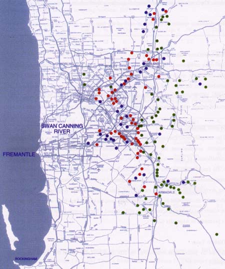 |
| Fig. 24. Final classification of sites. Red = Impacted (monitoring); Blue = Intermediate; Green = Reference. |
| (original size image) |
| Table 18. Diatom genera from urban streams and drains of Perth. | |
|---|---|
| Achnanthes | Luticola |
| Achnanthidium | Martyana |
| Amphora | Mastolgloia |
| Aneumastus | Melosira |
| Anomoeoneis | Meridion |
| Aulacoseira | Navicula |
| Bacillaria | Neidium |
| Brachysira | Nitzschia |
| Caloneis | Pinnularia |
| Camphylodiscus | Pleurosigma |
| Cocconeis | Rhopalodia |
| Craticula | Paralia |
| Ctenophora | Sellaphora |
| Cyclotella | Skeletonema |
| Cymbella | Stauroneis |
| Denticula | Staurosira |
| Diadesmis | Stenopterobia |
| Diploneis | Surirella |
| Encyonema | Synedra |
| Entomoneis | Tabellaria |
| Epithemia | Tabularia |
| Eunotia | Thalassionema |
| Fallacia | Thalassiosira |
| Fragilaria | Tryblionella |
| Frustulia | |
| Gomphonema | Total 53 |
| Gyrosigma | |
| Hantzschia | |
| Hyppodonta | |
| Table 19.Diatom species recorded from the urban streams and drains of Perth | ||
|---|---|---|
| Achnanthes | Eunotia | Neidium |
| A.brevipes | E.camelus | N.affine |
| Achnanthidium | E.curvata | N.productum |
| A.binodis | E.diodon | N.iridis |
| A.citronella | E.eurycephaloides | Nitzschia |
| A.delicatula | E.exigua | N.acicularis |
| A.exigua | E.flexuosa | N.acuminata |
| A.hauckiana | E.formica | N.amphibia |
| A.hungarica | E.incisa | N.closterium |
| A.lacunarum | E.monodon | N.dissipata |
| A.lanceolata | E.pectinalis | N.fasciculata |
| A.microcephala | E.trigibba | N.frustulum |
| A.minutissima | Fallacia | N.gracilis |
| A.oblongella | F.auriculata | N.hummi |
| A.plonensis | F.pygmeae | N.linearis |
| A.reidensis | Fragilaria | N.lorenziana |
| Amphora | F.brevistriata | N.obtusa |
| A.australiensis | F.capucina | N.palea |
| A.coffeaeformis | F.construens | N.palaecea |
| A.costellata | F.miniscula | N.scalaris |
| A.fontinalis | F.punctata | N.sigma |
| A.holsatica | F.rumpens | Paralia |
| A.obtusa | F.vaucheriae | P.sulcata |
| A.ovalis | Frustulia | Pinnularia |
| A.pediculus | F.anceps | P.borealus |
| A.veneta | F.megaliesmontana | P.braunii |
| A.ventricosa | F.rhomboides | P.divergens |
| Aneumastus | F.vulgaris | P.gibba |
| A.tusculus | Gomphonema | P.maior |
| Anomoeoneis | G.acuminatum | P.microstauron |
| A.sphaerophora | G.affine | p.subcapitata |
| Aulacoseira | G.angustatum | P.viridis |
| A.distans | G.intricatum | Pleurosigma |
| A.granulata | G.lanceolatum | P.decorum |
| Bacillaria | G.parvulum | P.elongatum |
| B.paxillifer | G.truncatum | P.formosum |
| Brachysira | G.undulatum | P.longum |
| B.serians | Gyrosigma | P.salinarum |
| B.styriaca | G.balticum | Rhopalodia |
| B.vitrea | G.distortum | R.brebissoni |
| Caloneis | G.kutzingii | R.gibba |
| C.bacillum | G.spencerii | R.gibburela |
| C.ventricosa | Hantzschia | R.musculus |
| Camphylodiscus | H.amphioxys | Sellaphora |
| C.clypeus | H.virgata | S.pupila |
| Cocconeis | Hyppodonta | Skeletonema |
| C.convexa | H.capitata | S.costatum |
| C.distans | Luticola | Stauroneis |
| C.placentula | L.mutica | S.acuta |
| C.scutellum | L.pseudomutica | S.anceps |
| C.sublittoralis | Martyana | S.dubitabilis |
| Craticula | M.martyi | S.pachycephala |
| C.cuspidata | Mastogloia | S.phoenicentron |
| C.halophila | M.braunii | S.spicula |
| Ctenophora | M.elliptica | Staurosira |
| C.pulchella | M.exigua | S.construens |
| Cyclotella | M.smithii | Stenopterobia |
| C.atomus | Melosira | S.sigmatella |
| C.menenghiniana | M.moniliformis | Surirella |
| C.stelligera | M.nummuloides | S.angusta |
| C.striata | M.varians | S.fluviicygnorum |
| Cymbella | Meridion | S.ovalis |
| C.lanceolata | M.circulare | S.tenera |
| C.microcephala | Navicula | Synedra |
| C.naviculiformis | N.accomoda | S.ulna |
| C.pusilla | N.angusta | Tabellaria |
| C.similis | N.bicephala | T.floculossa |
| C.tumida | N.cancellata | Tabularia |
| C.ventricosa | N.cincta | T.fasciculata |
| Denticula | N.clamans | T.tabulata |
| D.subtilis | N.comoides | Thalassionema |
| Diadesmis | N.cruezbergensis | T.nitzschiodes |
| D.confervacea | N.cryptocephala | Thalassiosira |
| Diploneis | N.directa | T.australis |
| D.chersonensis | N.elegans | T.weissflogii |
| D.ovalis | N.elginensis | Tryblionella |
| D.smithii | N.exigua | T.acuminata |
| D.vacillans | N.festiva | T.circumsuta |
| Encyonema | N.gastrum | T.apiculata |
| E.delicatulum | N.grimmei | T.victoriae |
| E.gracile | N.muticola | T.levidensis |
| E.mesianum | N.placentula | |
| E.minutum | N.punctata | |
| E.silesiacum | N.radiosa | |
| Entomoneis | N.ramosissima | |
| E.costata | N.robertsiana | |
| Epithemia | N.ryhnchocephala | |
| E.sorex | N.salinarum | |
| N.shoeterii | ||
| N.stigmatifera | ||
| N.subrhyncocephala | ||
| N.symmetrica | ||
| N.tripunctata | ||
| N.virudila | Total 211 | |
Urban streams have been used as an effective drainage system to dispose of water and effluents. Historically the function of urban streams was considered to be different from the rural streams. Therefore selecting a large number of reference sites (pristine sites) for a predictive model in any city in Australia is difficult. In winter, the urban drains and streams are prone to fast flow and scouring. In summer many of them may dry up. The streams and drains in the metropolitan city of Perth are under the control of the Water Corporation and local government councils. The Water and Rivers Commission and Department of Environmental Protection have the responsibility of regulating the effluent discharge into the Swan-Canning River system. Consultation with these bodies was the essential initial step taken before selecting the sampling sites for the current project. Lack of uniform natural substrates (e.g. pebbles) and the heterogeneous nature of substrates, prompted the use of the 'pheriphytometers' which proved to be most effective in obtaining uniform samples. The reference sites were mostly away from the inner city. In spite of these problems, the project achieved the objectives as specified in the introduction of this report.
Although three samplings covering close to 180 sites were carried out (1996-1997), the spring-summer (1997) samples of 146 sites with complete set of data were used for developing the predictive model. The 1996 summer-spring sampling was used to confirm the water quality characteristics of the sites. The 1997 autumn-winter sampling was also useful in confirming the status of the chosen sites, as well as to test the predictive model. However, winter may not be an ideal season for sampling the urban streams because of fast flow, scouring and flooding. The species diversity of diatoms was higher in winter because of the 'import' of species due to flooding. However the 'autochthonous' species were still there in winter in each site crucial in developing a predictive model. The seasonality of species was not a crucial factor in the distribution pattern of diatoms. Generally winter had a 'dilution effect' on water quality parameters. In order to maximise the representation from diverse urban stream habitats, natural streams and artificial streams including concrete drains, with widely differing catchment land use, were selected for sampling.
Use of artificial substrates (the JJ Periphytometers) proved to be an ideal way of overcoming the problem of heterogeneity of natural substrates present in the urban streams and drains. Loss of periphytometers due to vandalism or torrential storm flow could be offset to a greater degree by securing the periphytometer strongly as well as camouflaging them. The colourless periphytometer merges well with water. After loss of almost 25% of periphytometers during the first sampling, we were able to minimise the loss drastically in subsequent samplings (less than 10%). A second visit required to retrieve the sampler is often mentioned as a disadvantage. However, a second visit is very useful in confirming the water quality parameters and stream conditions. Moreover, the time required for installing the samplers is minimal. The trophic status of the sites can be determined by extraction of the Chlorophyll a and fresh cell count from the periphytometer. Rather than relying on a single measurement of Chlorophyll a from a water sample, the Chlorophyll extract from the periphytometer is a better measure of the trophic status of the site. The Chlorphyll extract and cell count could be standardised for determining the trophic status of a site. Several Chlorophyll extract measurements obtained in this project (not presented in the current report) confirm the potential for the use of the periphytometer as a sampler for determination of trophic studies. A snapshot of a trophic status of the streams could be obtained by the periphytometer sampling. The effectiveness of the sampling method was confirmed by a one year supplementary project (reported in Progress Report No. 5 of this project in 1999).
Physical perturbations may play an important role in disrupting the community structure of periphyton. Therefore we need to resolve issues such as how many samples should be collected from a site? Should we include both pools and riffles? In the supplementary investigation mentioned above, it was confirmed that there was no significant difference in community structures found between pool and riffle sites. Within stream variability was much less than variability between streams according to the results obtained. The duration of colonisation of the periphytometers is often another issue raised. Our trials in natural and highly impacted sites and reference sites (least impacted) indicated that two weeks is sufficient to obtain a representative sample, although at eutrophic sites, the colonisation was faster and a climax stable community was reached earlier than in pristine sites. The same investigation also confirmed that the periphytometers did collect both epiphytic and benthic diatoms.
'Clustering' all sites using UPGMA method is one of the most powerful ways of finding relationships among the sites. The initial rating of the sites as 'monitoring' (impacted) and reference is only a starting point. Historical data and visual observation on the integrity of the streams helped to initiate the basic classification of monitoring and impacted sites. Although there were more than 30 variables, seven of them proved to be most significant i.e. alkalinity, NH3, TKN, TN, SRP, TP and colour, the rest of the variables showed high colinearity.
River or stream health is defined as the chemical, physical and biological integrity of the aquatic system – a concept that refers to the natural structure and functions of the ecosystem (Karr 1999). The concept of good condition of a stream should therefore encompass habitat as well as water quality. It is the interaction of biogeographic and evolutionary processes in the regional, climatic and ecological context that determines the 'integrity' of an aquatic system. As urbanisation advances, landscapes of the catchment alters drastically affecting the biota of rivers and streams. The thirty environmental variables selected for the project as criteria for classification of the sites reflect the alteration to the catchment.
Considerable cross linearity has been found between the environmental factors selected for determining the status of the sites. Trophic status can be singled out as the most important factor determining the health of the Swan-Canning estuary (Swan River Trust 1999). The causes of eutrophication originate from the catchments. Traditionally the vast rural catchment of the Avon River – with its dryland agriculture has been focussed as the source of excessive nutrient loading. Subcatchments within the urban area have received relatively little attention. Environmental factors such as water table depth, riparian damage, loss of native vegetation, landfills and rubbish tips, and land use do contribute substantially to eutrophication. For example shalllow water table contributes to groundwater pollution. Exotic soft tissue plants decompose fast adding to the carbon, phosphorus and nitrogen supply to the rivers. Therefore it was not surprising that the seven factors – alkalinity, electrical conductivity, total phosphorus, total nitrogen, total organic nitrogen, soluble reduced phosphorus and colour had the maximum correlation with the sites. The dendrogram (hierarchal classification( separated the sites into 12 groups on the basis of these environmental variables. The hierarchal classification by the agglomerative hierarchial fusion method using flexible unweighted pair group means average (UPGMA) is a powerful method for grouping closely related sites together linking them to a large number of variables.
Although initially a large number of sites were allotted to 'pristine' (reference) status after analysis of the classification their status had to be reviewed. The initial status was mostly based on historical data of single measurements of nutrients, or visual observations of the condition of river banks and peripheral vegetation. The number of reference sites were reduced from 88 to 66 and impacted sites increased to 80 of which 18 were grouped as intermediate as a result of the review, Total N was correlated to TP and TP to SRP pointing to eutrophication so common in the wetlands and rivers of the Swan coastal plain.
The Principal Component Analysis Ordination of the sites with the environmental variables of nitrogen and phosphorus separated the reference sites from the monitoring sites (impacted sites), although there were one or two outliers (Figs. 15 & 16). Looking at the PCA of the environmental variables, it is clear that there is an area of intergradation between the two – reference and impacted. The sites between the two extremes can be described as 'the intermediate or mixed category'.
Subgroups within the hierarchal classification were further fused into larger groups in order to interpret the relationships among the sites (Tables 14 and 16). As a result of the fusion of subgroups there were mixed groups. A review of the sites in the mixed groups (mixture of reference and monitoring sites) re-examining the conditions of the sites resulted in the recognition of a third group – the intermediate.
The hierarchial grouping generated from the distribution pattern of diatoms basically followed the site classification based on environmental variables. Conceptually if the biomonitors reflect the stream conditions, then a classification based in biomonitors should follow that based on environmental variables. Further, if the autecology of the biomonitors is known, the species assemblages present in each site or group of sites, may provide more information about the stream conditions even beyond what is measured by environmental variables. The strength of diatoms as powerful biomonitors has been confirmed yet again by the present research.
Diatom assemblages of the sites are grouped into clusters according to their similarity. This results in diatoms of similar ecological preferences being grouped together. A perusal of Figure 19 clearly shows how the vast majority of the reference sites were separated into groups 10 to 12 and most of the monitoring sites in groups 1,2,6,7,8 and 9 and then there are the mixed groups containing both reference and monitoring groups. A close analysis of the conditions in these mixed sites indicate these sites are characterised by varying impacts on peripheral vegetation and ecological integrity. Discriminant Function Analysis, mostly validated the classification of sites based on diatom taxa. The high degree of concordance between the two types of classification of sites is evident in the results (Tables 8 and 9). When three classes of stream status is recognised ie. Reference, Monitoring and Intermediate, the rate of successfully predicting the group membership by environmental data was 86.3%.
Multidimensional scaling used as an ordination method with diatom species and correlation of environmental factors generated Biplots summarising the relationship between diatom distribution patterns and the status of the sites. The reference sites are separated clearly towards the right and the monitoring towards the left and then there are the intermediate types (Figs. 20 –23) (subgroups 9, 4 and 5) in the UPGMA classification. Only diatom species with the highest correlation with the ordination are shown (Fig. 20) which are the indicator species. Synedra ulna, Achnanthidium oblongella, Achnanthidium minutissima and Eunotia pectinalis are among the species indicating a strong distribution pattern with the reference sites. On the other hand, Achnanthidium exigua, Fragilaria brevistriata, Bacillaria paxillifer, Hyppodonta capitata and Staurosira construens are the indicator species with high correlation with the monitoring sites.
The environmental factors with high correlation coefficient with the ordination clearly distinguish those associated with the reference sites from the monitoring sites (Fig. 21). Percentage of native vegetation and water table depth are highly correlated with the reference sites. Alkalinity, ground water salinity, intense catchment land use, riparian damage and colour of water are highly correlated with impacted sites as indicated by diatom distribution (Table 12)
Thus the biomonitors – the diatoms clearly identify the status of stream conditions beyond water quality. Other relevant stream conditions associated with distribution were, distance from the estuary and electrical conductivity.
Initially allotted condition status of the sampling sites based on historical data and observations of the stream conditions, have been mostly confirmed and further modified as a result of the present investigation. The classification of the sites based on both environmental variables and diatom distribution confirmed the classification of the sites into three categories, Reference (relatively pristine), Monitoring (impacted) and Intermediate (mixed groups) (Table 14 & Fig. 24).
The location of most of the relatively pristine sites is away from the estuary and its tributaries. The native vegetation is less impacted in these sites and soil type is mostly clay, which tends to bind phosphorus. The water table is deeper with less chance of ground water contamination. The diatom assemblages associated with these conditions clearly separated the reference sites from the rest.
On the other hand, the monitoring sites are located proximal to the estuary and its tributaries. The sandy soil in these sites favour easy leaching of phosphorus; the native vegetation is replaced by soft tissue exotic species, the water table is deeper favouring ground water contamination. The proximal sites are prone to maximum impact of urbanisation – described in Chapter 2. High nutrient input by the urban catchment disproportionate to catchment area, to the estuary has been documented before (Swan River Trust 1994, 1996, 1999). Industries, landfills and rubbish tips and sewerage drains are all located proximal to the Swan Canning River estuary.
However, the demarcation of reference sites and monitoring sites is not very clear cut. There are a few sites affected by agricultural, horticultural and farming impact in the Ellen Brook catchment as well as Southern River. This project has been able to gather data on close to 160 sites covering an area of 1500 km2 around the metropolitan city of Perth. The recognition of an Intermediate category is of great relevance to the management strategy. Design of wetlands to strip extra nutrients discharged into the Rivers through the urban drains and streams, revegetation of banks and streams, eradication of weeds and prevention of soil erosion and rehabilitation measures to bring 'life' back to the urban streams and a host of other measures currently being undertaken by Urban Catchment Groups (Swan River Trust 1999) should be focussed on the sites identified in this project as Impacted and Intermediate. Eutrophication of the Swan-Canning River estuary may be reversed by appropriate actions focussing on impacted urban streams and drains.
Biomonitoring using diatoms may be introduced as part of the management strategy to measure the success of rehabilitation and restoration that may be introduced.
The distribution pattern of diatoms constrained on the site groups forming two way table, enable the analysis of species assemblages by sites as well as site groups by species. A glimpse of the table (Table 10) gives an overview of the grouping of diatom species in relation to the sites. The sites towards the right are mainly monitoring, with assemblages of indicator species of healthy conditions of the streams. On the other hand on the left of the table, there is a cluster of indicators of impacted conditions.
This table can be used to assess the health of any 'test' site. Data on assemblages of diatoms from a 'test' site (relative frequency of dominant species) can be added to the table and depending on the composition of the assemblage, the 'test' site may be classified with reference or impacted. This two way table is a potential predictor of the condition of the stream.
Following Wright (1995), a diatom index was developed using discriminant function analysis with the software program SPSS 7.1. The index is based on the test site having indicator species for reference sites versus 'non indicator' species (unexpected). Any site with data on the relative frequency of diatom assemblages and can be tested for the status of the site. This model has been derived from the diatom species in the Perth metropolitan streams but has the potential to be applied in other parts of Australia.
The two way table and the predictive model both could be applied to test sites in other parts of Australia as well. There is remarkable similarity of diatom species present in the urban streams and the rivers and streams of the south west of Western Australia. The vast majority of the species (>90%) are common to both regions. The difference is predominantly due to difference in community structure. There are much more pristine sites in the native forests of the south west compared to the Perth region and therefore there is higher diversity of indicator species of references sites in the south west of Western Australia than in the urban sites e.g. species of Eunotia. On the other hand, there is a high diversity of diatom species indicating impacts such as salinisation and eutrophication and acidification in the south west than in the Perth urban area as well, e.g. species of Mastogloia, Amphora, Hyalodiscus.
However, diatoms are more universal in their distribution than macroinvertebrates and these models developed in a temperate region such as those in this project may be adapted to use in other temperate regions of Australia with ease.
Once the regional diatom flora has been investigated, it is relatively simple to adapt the above two techniques to assess the urban stream health elsewhere on a regional basis, using the two way table as well as the diatom index developed in this project. If these tools are supplemented with information on the autecology of dominant species, biomonitoring may be used not only for mere assessment but also for diagnosis of specific maladies.
WATER COURSE: Claisebrook Drain DRAINAGE: Swan River
SITE: Macey St, East Perth. GPS COORDINATES: 394.0 E 6464.2 N
URBAN CODE: URB 061 (Monitoring site) SITE NUMBER: 042
DISTANCE FROM ESTUARY: Okm WATER TABLE DEPTH: 1-2m
| Season | Width (metres) | Depth (metres) | pH | Conductivity (ms/cm) |
| Spring-Summer 1997 | 60 | 3 | 8.60 | 0.72 |
| Autumn-Winter 1997 | 60 | 0.12 | 8.00 | 0.64 |
NOTES: This permanent, concrete section of the Claisebrook Main Drain has recently been developed from an open drain, to an almost harbour-like structure, with a direct outlet into the Swan River. Submerged plant life consists almost totally of filamentous algae, which inhabit the limestone rock lining the edges of the drain. No emergent vegetation is present at this site. The autumn-winter 1997 sampling site was slightly upstream where there is less mixing with brackish river water. The surrounding land use is light industrial and residential.
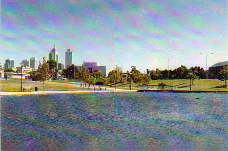
Site 042. Autumn-winter 1997.
WATER COURSE: Mills St Main Drain DRAINAGE: Canning River
SITE: Channon Rd, Bentley. GPS COORDINATES: 32o00'27'', 115o55'47"
URBAN CODE: URB 090 (Monitoring site) SITE NUMBER: 058
DISTANCE FROM ESTUARY: 2.4km WATER TABLE DEPTH: 1-2m
| Season | Width (metres) | Depth (metres) | pH | Conductivity (ms/cm) |
| Spring-Summer 1997 | 1.5 | 0.5 | 7.06 | 0.7 |
| Autumn-Winter 1997 | 2 | 0.4 | 7.00 | 0.38 |
NOTES: The area to the north-west of this urban stream is light industrial, while the area to the south~east is urban housing. This permanent section of the drain is immediately surrounded by cleared land. Only weeds and grasses surround the drain, and there is no submerged vegetation, although filamentous algae are dense in the water column. Site was more dominated by Kikuyu grass in autumn-winter 1997.
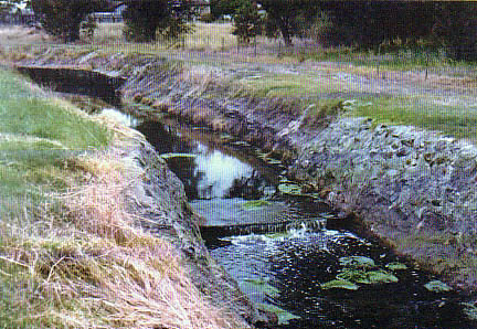
Site 058. Spring/summer 1997.
WATER COURSE: Brook St Main Drain DRAINAGE: Swan River
SITE: North Rd, Bassendean. GPS COORDINATES: 31o54"12', 115o57"29'
URBAN CODE: URB 045 (Monitoring site) SITE NUMBER: 040
DISTANCE FROM ESTUARY: 0.2km WATER TABLE DEPTH: 1-2m
| Season | Width (metres) | Depth (metres) | pH | Conductivity (ms/cm) |
| Spring-Summer 1997 | 1.5 | 0.3 | 7.3 | 0.60 |
| Autumn-Winter 1997 | 1.5 | 0.4 | 7.31 | 1.61 |
NOTES: Grasses and Eucalypts are the most common vegetation lining this permanent urban/residential drain. Some surface scum is visible. Suff ounding areas are composed of urban housing, a shopping centre, a bowling green and a football oval. Substrate is sandy. The Kikuyu grass had regrown near the bank in autumn-winter 1997 and the water was slightly more saline.
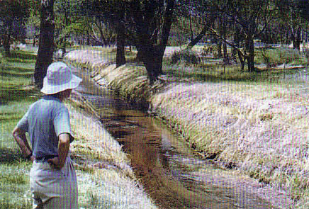
Site 040. Spring/summer 1997.
WATERCOURSE: Swan River Tributary DRAINAGE: Swan Estuary
SITE: Great Northern Highway Bridge, Upper Swan. GPS COORDINATES: 31o46"57', 116o01'21"
URBAN CODE:URB 003 (Monitoring Site). SITE NUMBER: 003
DISTANCE FROM ESTUARY: 0km WATER TABLE DEPTH: >5 m
| Season | Width (metres) | Depth (metres) | pH | Conductivity (ms/cm) |
| Spring-Summer 1997 | 20 | 2 | 8.9 | 7.5 |
| Autumn-Winter 1997 | 20 | 0.3 | 7.6 | 8.63 |
NOTES: This semi rural section of the river is permanent, and has a fairly rapid flow. The northern bank supports natural bushland, including Melaleuca sp., Eucalyptus sp., Acacia sp. and Pennisetum clandestinum (Kikuyu Grass), while the landuse on the southern bank is vineyards. Some emergent sedges are present in the shallow shore regions, the substrate of which is sandy. An increase in river flow was observed in autumn-winter 1997 with a decrease in pH and increase in conductivity.
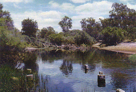
Site 003. Spring/summer 1997
WATER COURSE: Wyong Rd B. Drain DRAINAGE: Canning River
SITE: Fern Road, Wilson. GPS COORDINATES: 32o01'07", 115o55"17'
URBAN CODE: URB 091 (Monitoring site) SITE NUMBER: 059
DISTANCE FROM ESTUARY: 0.5km WATER TABLE DEPTH: 1-2m
| Season | Width (metres) | Depth (metres) | pH | Conductivity (ms/cm) |
| Spring-Summer 1997 | 3 | 0.5 | 7.00 | 0.68 |
| Autumn-Winter 1997 | 2.5 | 0.31 | 6.95 | 0.67 |
Season	Width	Depth	pH	Conductivity
	(metres)	(metres)		(MS/CM)

Spring-Summer	3	0.5	7.00	0.68
1997
Autumn-Winter	2.5	0.31	6.95	0.67
1997
NOTES: This urban drain runs from an urban reserve and aquatic centre, through another two parks and a small area of urban housing, to its outlet in Wilson Park Swamp. Eucalyptus trees line the banks of this permanent drain, which has a sandy substrate. Medium to high densities of submerged vegetation occurs, including Potamogeton sp. and Hydrilla sp. This site was in a similar condition in both sampling seasons.
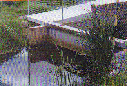
Site 059. Auturnn-winter 1997.
WATER COURSE: Binley Brook B. Drain DRAINAGE: Canning River
SITE: Ladywell St, Beckenham. GPS COORDINATES: 32o02'02", 115o57'32"
URBAN CODE: URB 095 (Monitoring site) SITE NUMBER: 063
DISTANCE FROM ESTUARY: 5.6km WATER TABLE DEPTH: 1-2m
| Season | Width (metres) | Depth (metres) | pH | Conductivity (ms/cm) |
| Spring-Summer 1997 | 1.5 | 0.2 | 7.71 | 1.13 |
| Autumn-Winter 1997 | 1.5 | 0.34 | 7.10 | 0.40 |
NOTES: This site, located in the middle of a light urban area, passes through an area of parkland and a small drainage pond on its lkm journey to the Canning River. A medium density of submerged macrophytes area present, while the only emergent species are generally exotic terrestrials. Sections of this permanent drain are partially concrete, while the remainder has a sandy substrate. This site was in a similar condition in both sampling seasons except for a slight drop in pH and conductivity.
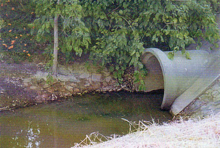
Site 063. Autumn-winter 1997.
WATER COURSE: Canning River DRAINAGE: Canning River
SITE: McNess Dve Bridge, Roleystone. GPS COORDINATES: 32o07'36", 116o06'04"
URBAN CODE: URB 155 (Reference Site). SITE NUMBER: 124
DISTANCE FROM ESTUARY: 33.2km WATER TABLE DEPTH: >5m
| Season | Width (metres) | Depth (metres) | pH | Conductivity (ms/cm) |
| Spring-Summer 1997 | 3 | 0.4 | 6.4 | 0.34 |
| Autumn-Winter 1997 | 3 | 0.37 | 6.0 | 0.27 |
NOTES: A small vineyard is located 500m upstream of this semi-rural section of the river. The substrate at this site is sand/clay and pebbly. Melaleuca sp. and a variety of grasses and exotic vegetation surround this site. No submerged vegetation is present. This site is located 15m upstream of a feeder stream, which originates in a large area of natural bushland. There was no significant difference in autumn/winter 1997.
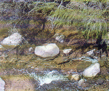
Site 124, Spring/summer 1997
WATER COURSE: Unnamed Stream DRAINAGE: Helena River
SITE: O'Connor Rd, Shire of Mundaring. GPS COORDINATES: 31o56'13", 116o08'05"
URBAN CODE: URB 059 (Reference Site). SITE NUMBER: 088
DISTANCE FROM ESTUARY: 23.5km WATER TABLE DEPTH: >5m
| Season | Width (metres) | Depth (metres) | pH | Conductivity (ms/cm) |
| Spring-Summer 1997 | 0.5 | 0.25 | 6.8 | 0.67 |
| Autumn-Winter 1997 | 0.5 | 0.26 | 6.1 | 0.5 |
NOTES: This rural stream has its source in the Darling Scarp foothills, and flows through an area of natural bushland and national park before reaching the Helena River. There was a significant drop in pH and conductivity in autumn/winter 1997.
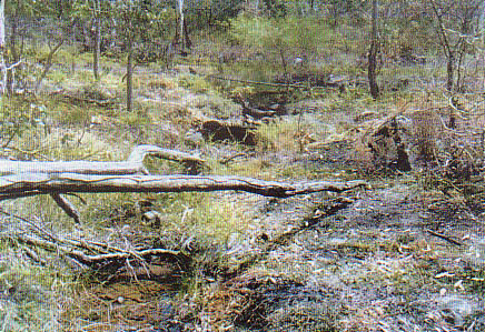
Site 088, Spring/summer 1997
Physico-Chemical Data Sheet spring/summer 1997
Appendix 2a Diatom Data Set
Correlation Coefficients of Diatom Species from SSH Ordination (autumn/winter 1997)
Correlation Coefficient (r > 0.4) of diatom species, sampled during autumn/winter with vectors from SSH ordination. P values were derived from 499 Monte Carlo random simulations of each diatom species
| Variable | Correlation Coefficient and P-value | Site status most closely associated with species vector |
| Achnanthidium minutissima | 0.762 (P < 0.05) | Reference |
| Eunotia pectinalis | 0.652 (P < 0.05) | Reference |
| Gomphonema angustatum | 0.641 (P < 0.05) | Reference |
| Cymbella similis | 0.570 (P < 0.05) | Reference |
| Synedra ulna | 0.563 (P < 0.05) | Reference |
| Achnanthidium binodis | 0.548 (P < 0.05) | Reference |
| Fragilaria rumpens | 0.525 (P < 0.05) | Reference |
| Cymbella microcephala | 0.460 (P < 0.05) | Reference |
| Fragilaria miniscula | 0.443 (P < 0.05) | Reference |
| Eunotia curvata | 0.436 (P < 0.05) | Reference |
| Navicula radiosa | 0.428 (P < 0.05) | Reference |
| Achnanthidium microcephala | 0.423 (P < 0.05) | Reference |
| Brachysira serians | 0.415 (P < 0.05) | Reference |
| Gomphonema intricatum | 0.411 (P < 0.05) | Reference |
| Achnanthidium exigua | 0.711 (P < 0.05) | Impacted |
| Fragilaria brevistriata | 0.703 (P < 0.05) | Impacted |
| Staurosira construens | 0.673 (P < 0.05) | Impacted |
| Diadesmis confervaceae | 0.640 (P < 0.05) | Impacted |
| Cyclotella meneghiniana | 0.634 (P < 0.05) | Impacted |
| Bacillaria paxillifer | 0.587 (P < 0.05) | Impacted |
| Hyppodonta capitata | 0.521 (P < 0.05) | Impacted |
| Diploneis ovalis | 0.479 (P < 0.05) | Impacted |
| Melosira varians | 0.451 (P < 0.05) | Impacted |
| Cocconeis placentula | 0.417 (P < 0.05) | Impacted |
| Amphora ovalis | 0.40 (P < 0.05) | Impacted |
Correlation Coefficients (r .> 0.4) of the environmental variables, measured during autumn/winter with the SSH ordination. P values were derived from 499 Monte Carlo random simulations of each variable.
| Environmental Variable | Correlation Coefficient and P-value | Site status most closely associated with parameter vectors |
| % Native Vegetation | 0.681 (P < 0.01) | Reference |
| Water Table Depth (m) | 0.681 (P < 0.01) | Reference |
| Distance from Estuary (km) | 0.6 (P < 0.01) | Reference |
| Catchment Soil Type (1-3) | 0.717 (P < 0.01) | Impacted |
| Riparian Damage (1-5) | 0.605 (P < 0.01) | Impacted |
| Catchment Land Use (1-5) | 0.585 (P < 0.01) | Impacted |
| NO3 (mg/l) | 0.563 (P < 0.01) | Impacted |
| NH3 (mg/l) | 0.549 (P < 0.01) | Impacted |
| Ground Water Salinity (mg/l) | 0.536 (P < 0.01) | Impacted |
| Alkalinity (mg/l) | 0.505 (P < 0.01) | Impacted |
| Temperature (° C) | 0.469 (P < 0.01) | Impacted |
| pH | 0.436 (P < 0.01) | Impacted |
| Visibility of Water (1-5) | 0.425 (P < 0.01) | Impacted |
Correlation Coefficient (r > 0.4) of diatom species, sampled during autumn/winter with vectors from SSH ordination. P values were derived from 499 Monte Carlo random simulations of each diatom species
| Variable | Correlation Coefficient and P-value | Site status most closely associated with species vector |
| Achnanthidium minutissima | 0.762 (P < 0.05) | Reference |
| Eunotia pectinalis | 0.652 (P < 0.05) | Reference |
| Gomphonema angustatum | 0.641 (P < 0.05) | Reference |
| Cymbella similis | 0.570 (P < 0.05) | Reference |
| Synedra ulna | 0.563 (P < 0.05) | Reference |
| Achnanthidium binodis | 0.548 (P < 0.05) | Reference |
| Fragilaria rumpens | 0.525 (P < 0.05) | Reference |
| Cymbella microcephala | 0.460 (P < 0.05) | Reference |
| Fragilaria miniscula | 0.443 (P < 0.05) | Reference |
| Eunotia curvata | 0.436 (P < 0.05) | Reference |
| Navicula radiosa | 0.428 (P < 0.05) | Reference |
| Achnanthidium microcephala | 0.423 (P < 0.05) | Reference |
| Brachysira serians | 0.415 (P < 0.05) | Reference |
| Gomphonema intricatum | 0.411 (P < 0.05) | Reference |
| Achnanthidium exigua | 0.711 (P < 0.05) | Impacted |
| Fragilaria brevistriata | 0.703 (P < 0.05) | Impacted |
| Staurosira construens | 0.673 (P < 0.05) | Impacted |
| Diadesmis confervaceae | 0.640 (P < 0.05) | Impacted |
| Cyclotella meneghiniana | 0.634 (P < 0.05) | Impacted |
| Bacillaria paxillifer | 0.587 (P < 0.05) | Impacted |
| Hyppodonta capitata | 0.521 (P < 0.05) | Impacted |
| Diploneis ovalis | 0.479 (P < 0.05) | Impacted |
| Melosira varians | 0.451 (P < 0.05) | Impacted |
| Cocconeis placentula | 0.417 (P < 0.05) | Impacted |
| Amphora ovalis | 0.40 (P < 0.05) | Impacted |
List of the most common diatom species, sampled in Autumn/winter, present in at least 40% of the sites in each group ordered by declining frequency of occurrence.
| Gp. 1 (25) | % | Gp. 2 (28) | % | Gp. 3 (37) | % | Gp. 4 (58) | % |
| Staurosira construens | 92 | Nitzschia palea | 96 | Achnanthidium exigua | 95 | Eunotia pectinalis | 97 |
| Nitzschia palea | 92 | Synedra ulna | 79 | Cyclotella meneghiniana | 97 | Synedra ulna | 90 |
| Synedra ulna | 92 | Gomphonema parvulum | 75 | Fragilaria brevistriata | 89 | Achnanthidium minutissima | 89 |
| Eunotia pectinalis | 88 | Achnanthidium oblongella | 75 | Nitzschia palea | 84 | Nitzschia palea | 76 |
| Sellaphora pupila | 84 | Navicula accomoda | 71 | Staurosira construens | 81 | Gomphonema angustatum | 74 |
| Navicula cryptocephala | 76 | Bacillaria paxillifer | 65 | Diadesmis confervaceae | 76 | Navicula accomoda | 69 |
| Gyrosigma kutzingii | 76 | Fragilaria brevistriata | 64 | Navicula accomoda | 73 | Achnanthidium oblongella | 64 |
| Navicula virudila | 76 | Achnanthidium lanceolata | 61 | Gomphonema parvulum | 65 | Cymbella similis | 60 |
| Achnanthidium minutissima | 76 | Cyclotella meneghiniana | 61 | Sellaphora pupila | 65 | ||
| Ctenophora pulchella | 74 | Achnanthidium minutissima | 65 | ||||
| Fragilaria brevistriata | 72 | Ctenophora pulchella | 62 | ||||
| Nitzschia frustulum | 72 | ||||||
| Cyclotella meneghiniana | 68 | ||||||
| Bacillaria paxillifer | 68 |
 Riversinfo Australia (au.riversinfo.org): Publication Information:
Current at December 2002
![]() au.riversinfo.org has been developed to facilitate public access to scientific and technical information on Australia's Rivers. Much of this material was paid for using public funds and is therefore owned by the Australian people. Environment Australia have been instrumental in making available all the publications from:
au.riversinfo.org has been developed to facilitate public access to scientific and technical information on Australia's Rivers. Much of this material was paid for using public funds and is therefore owned by the Australian people. Environment Australia have been instrumental in making available all the publications from:
 The au.riversinfo.org Internet site is in-part supported by the Natural Heritage Trust. The Natural Heritage Trust focuses on five key environmental themes - land, vegetation, rivers, coasts and marine, and biodiversity. The programs of the Natural Heritage Trust play a major role in developing sustainable agriculture and natural resource management, as well as protecting our unique biodiversity through improved management and delivery of resources.
 The au.riversinfo.org Internet site is in-part supported by Sydney Airport who have co-funded a Natural Heritage Trust supported project intended to develop Internet based environmental information integration and management systems. This will assist in developing an overall perspective on the demands and uses for environmental resources